map_path

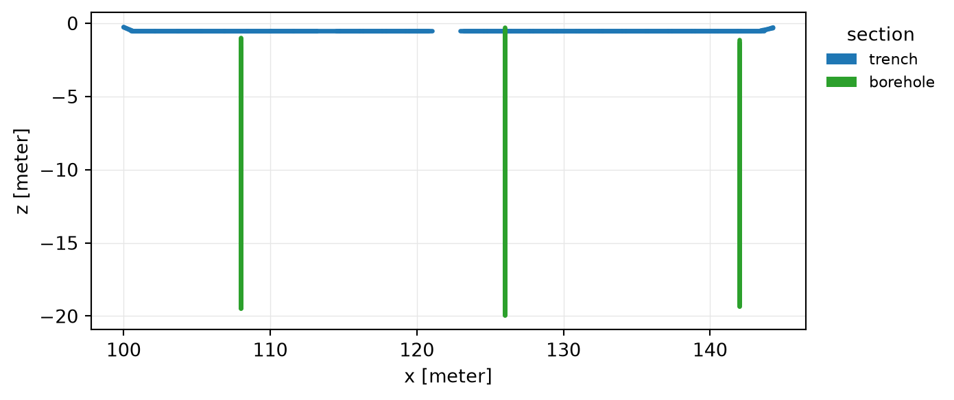
map_path(
    inventory: ‘Inventory’ ,
    optical_path: ‘str | OpticalPath | None’ = None,
    acquisition_key: ‘str | None’ = None,
    time: ‘timeable_types | None’ = None,
    x: ‘str | None’ = None,
    y: ‘str | None’ = None,
    color: ‘str’ = distance,
    n_samples: ‘int’ = 1000,
    cmap: ‘str’ = viridis,
    linewidth: ‘float’ = 2.5,
    aspect: ‘str | float | None’ = None,
    ax: ‘plt.Axes | None’ = None,
    legend: ‘bool’ = True,
    show: ‘bool’ = False,
)-> ‘plt.Axes’

Plot where an inventory’s fiber physically goes.

The polyline is the path’s geometry read through the inventory’s coordinate reference system. Stretches which state no position are left out rather than bridged, so a slack coil or an unsurveyed run reads as the gap it is.

With no path named this draws every path which places itself, since a map of one cable in an inventory of several is a strange default.

Parameters

Parameter	Description
inventory	The inventory to draw.
optical_path	A path address, name, or object; None draws all of them.
acquisition_key	Resolve one path from an acquisition key instead.
time	The instant to resolve at.
x, y	The CRS axes to draw, defaulting to the first two the CRS declares. A borehole needs that default overridden: a hole runs straight down, so a plan view collapses it to a point.
color	“distance”, a geometry column, a label group, or “coupling”.
n_samples	How finely the path is sampled.
cmap	Colormap for a continuous coloring.
linewidth	Width of the drawn fiber.
aspect	Axes aspect; None picks equal when both axes share units.
ax	An Axes to draw on.
legend	Whether to draw the legend or colorbar.
show	Whether to call plt.show.

Examples

import dascore as dc
from dascore.viz.inventory import map_path

inventory = dc.get_example_inventory("tunnel")
_ = map_path(inventory, x="x", y="z", color="section")