These notes provide the reasoning for DASCore’s fourier module implementation.
Summary
For output="FFT", DASCore multiplies NumPy’s FFT coefficients by the coordinate spacing along each transformed dimension in order to:
Produce the same units as the continuous fourier transform
Preserve the continuous-transform form of Parseval’s identity
Ensure the zero-frequency coefficient approximates the integral of the signal
output="AS", "PS", and "PSD" convert those coefficients into amplitude, power, and power-spectral-density representations. Their normalization uses the DFT domain extent \(n\,dx\), not merely the endpoint span \((n-1)\,dx\).
Continuous Fourier Transform
The Continuous Fourier Transform (CFT) can be defined as:
Let us consider how \(F\) affects the units of \(f(x)\) by first examining the units of the transformed variable \(\xi\). Since the product of the variables in the exponential (\(i 2 \pi \xi x\)) must be unit-less, and \(2 \pi i\) have no units, it follows that the units of \(\xi\) must be the multiplicative inverse of the units of \(x\). That is, if the units of \(x\) are seconds(\(s\)), the units of \(\xi\) must be \(\frac{1}{s} = Hz\). This is confirmed by rudimentary experience with time series analysis.
The units of \(\hat{f}\) are also straight-forward to ascertain from Equation 1. Because \(e^{-i 2 \pi \xi x}\) has no units, the resulting units of \(\hat{f}\) are just the units of \(f(x)\) multiplied by the units of \(dx\). So, if the original units of \(f\) are in volts (\(V\)) and the units of \(x\) are seconds, the units of \(\hat{f}\) are \(Vs\), which is often written as \(\frac{V}{Hz}\).
One property of Equation 1 relevant to DASCore’s implementation is Parseval’s identity which, in 1D, can be stated as:
Loosely speaking, we might say that the energy of the function is preserved by the transform.
A related property of Equation 3 is that the zero frequency represents the DC offset, or integral, of the original function. Setting \(\xi=0\) in Equation 1 we see:
Before defining the Discrete Fourier Transform (DFT), let’s first consider how we expect DASCore’s DFT to behave based on Equation 1 and the discussion in the previous section.
Units: The transformed axis should have inverse units of the original axis, and the data units should be multiplied by the units of the pre-transform dimension.
Energy Preservation: From Equation 3, integrating the square of the untransformed data should yield the same value as integrating the square of the amplitude spectra.
The amplitude of the zero frequency should be equal to the integral of the signal.
Now, let’s look at Numpy’s DFT, which is defined as:
where \(a\) is the untransformed series of length \(n\), \(A\) is the transformed discrete series with elements corresponding to frequency bins (\(k\), \(k=0, ..., n-1\))
Right away you might notice some reasons Equation 4 can’t meet our expectations. First, nowhere are the units of \(a\)’s axis multiplied in the summation. Since the exponential term must be unit-less, \(a\) must have the same units as \(A\). Next, the energy can’t be preserved since the number of elements in the summation increases as \(n\) increases. Lastly, \(A(0) = \sum_{m=0}^{n-1} a_m\) which is not the integral, but the sum, of \(a\) (it doesn’t consider sample spacing).
Two Sine Waves
To illustrate some of these issues, consider a sine wave with amplitude of \(\pm\)\(b_0\) and dominant frequency of \(f_0\) Hz.
\[
f(x) = b_0 sin(2 \pi\ f_0 x)
\tag{5}\]
We know (or can derive/look up) the CFT of this function:
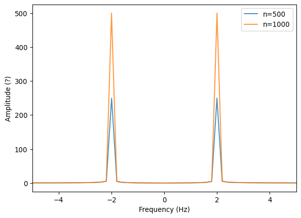
To discretize Equation 5, let \(f_0 = 2\), the total signal duration (\(T\)) = 5 seconds, and \(b_0\) = 1. We create two sine waves, one with 500 samples and one with 1000 samples. When we naively perform the dft, shift the zero frequency to the center, and plot the amplitude spectra we get the following:
Code
import matplotlib.pyplot as pltimport numpy as npdef get_sine_and_time(duration, freq, samples, amplitude=1):"""Return an array of time, sine with specified parameters""" time = np.linspace(0, duration, num=samples) sin = amplitude * np.sin(2* np.pi * freq * time)return time, sindef get_fft_and_freqs(time, signal):"""return the fft and corresponding frequencies of a signal""" fft = np.fft.fft(signal) dt = time[1] - time[0] # assuming evenly sampled freqs = np.fft.fftfreq(len(time), dt)return np.fft.fftshift(freqs), np.fft.fftshift(fft)def plot_amplitude_spectra(freqs1, fft1, freqs2, fft2, lims=(-5, 5)):"""plot amplitude spectra without normalization""" plt.plot(freqs1, np.abs(fft1), label=f"n={len(freqs1)}", alpha=0.8) plt.plot(freqs2, np.abs(fft2), label=f"n={len(freqs2)}", alpha=0.8) plt.xlabel("Frequency (Hz)") plt.ylabel("Amplitude (?)") plt.xlim(*lims) plt.legend()return plt.gca()duration =5# secondsfreq =2# Hzn1, n2 =500, 1000# number of samples# get two cases, one with 100 and 300 samplest1, sin1 = get_sine_and_time(duration, freq, n1)t2, sin2 = get_sine_and_time(duration, freq, n2)# get their transformsfreqs1, fft1 = get_fft_and_freqs(t1, sin1)freqs2, fft2 = get_fft_and_freqs(t2, sin2)# and plotax = plot_amplitude_spectra(freqs1, fft1, freqs2, fft2)plt.show()
Figure 1: Sine amplitude spectrum
As expected, both outputs have spikes at \(\pm f_0\) (2Hz), but the amplitude of the 1000 sample function is 2X larger than the 500 sample function. This isn’t entirely surprising; from Equation 6 we expect the amplitude to tend toward infinity as the signal moves from discrete to continuous (\(n \rightarrow \infty\)). However, this scaling is typically not useful. Certainly, it won’t meet our expectations stated above.
Scaling
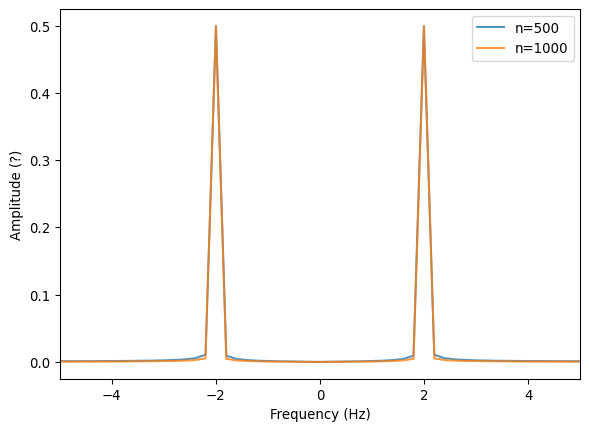
One approach to fix scaling discrepancy is to divide each amplitude spectrum by the number of samples. After which, they have nearly identical spectral amplitudes.
A nice result of this approach is that the amplitude-spectrum magnitude at \(\pm\) the dominant frequency (\(f_0\)) is half the amplitude of the original sine wave (\(b_0\)) for a full two-sided transform. Folding negative-frequency magnitude onto its positive-frequency partner recovers \(b_0\).
However, does the equivalent of Equation 3 hold if we perform numerical integration?
Code
import numpy as npdef integrate_amp_squared(x, signal):"""Integrate the square of the abs of signal with x coordinates.""" dx = x[1] - x[0] # x must be evenly sampled. amp_sq = np.abs(signal) **2return np.trapezoid(amp_sq, dx=dx)# Check for first sine wavefft1_energy = integrate_amp_squared(freqs1, n_scaled_fft1)time1_energy = integrate_amp_squared(t1, sin1)print(f"sine wave (n={len(t1)}) energy {time1_energy:.02f}")print(f"fft n-scaled (n={len(t1)}) energy {fft1_energy:.02f}")# Then secondfft2_energy = integrate_amp_squared(freqs2, n_scaled_fft2)time2_energy = integrate_amp_squared(t2, sin2)print(f"sine wave (n={len(t2)}) energy {time2_energy:.02f}")print(f"fft n-scaled (n={len(t2)}) energy {fft2_energy:.02f}")
sine wave (n=500) energy 2.50
fft n-scaled (n=500) energy 0.10
sine wave (n=1000) energy 2.50
fft n-scaled (n=1000) energy 0.10
It doesn’t. And what about the units? As we saw above, \(A\) in Equation 4 would have the same units as \(a\).
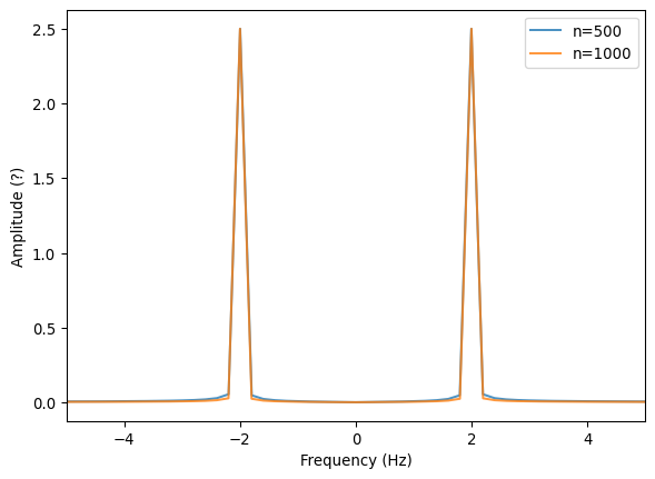
What if, drawing inspiration from Equation 1, we simply scale the output by the function’s sample spacing (\(dx\))? For an \(n\)-sample DFT, the periodic-domain extent that determines the frequency-bin spacing is
As expected, the transforms with different numbers of points still have the same magnitude at \(\pm f_0\). Checking their energy conservation:
Code
# Check for first sine wavefft1_energy = integrate_amp_squared(freqs1, dt_scaled_fft1)time1_energy = integrate_amp_squared(t1, sin1)print(f"sine wave (n={len(t1)}) energy {time1_energy:.02f}")print(f"fft dt_scaled (n={len(t1)}) energy {fft1_energy:.02f}")# Then secondfft2_energy = integrate_amp_squared(freqs2, dt_scaled_fft2)time2_energy = integrate_amp_squared(t2, sin2)print(f"sine wave (n={len(t2)}) energy {time2_energy:.02f}")print(f"fft dt_scaled (n={len(t2)}) energy {fft2_energy:.02f}")
sine wave (n=500) energy 2.50
fft dt_scaled (n=500) energy 2.50
sine wave (n=1000) energy 2.50
fft dt_scaled (n=1000) energy 2.50
The continuous-transform form of energy conservation is recovered, and the expected units are produced. Dividing coefficient magnitudes by the DFT extent \(T_{DFT}\) gives amplitudes in the original data units (Equation 7).
Zero Frequency
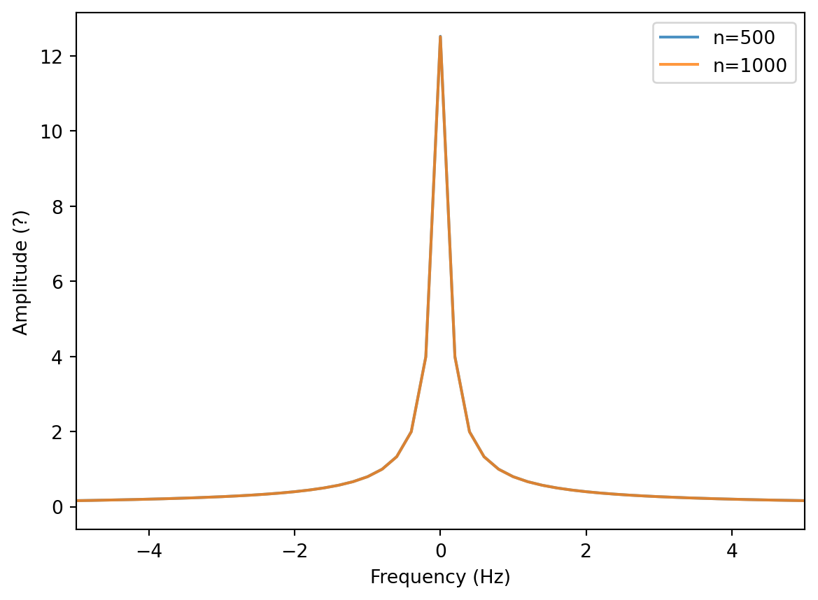
What about the zero frequency representing the integral over the signal domain? It is hard to say with a zero-mean signal like the sine wave used in the previous section. However, we could use a ramp function, such that \(f(x) = x\). Using the 5 second signal from before, which forms a triangle with area of 12.5, we get the following transforms:
NumPy coefficients multiplied by the product of transformed-axis sample spacings
Complex continuous-transform coefficients; data units are multiplied by the original coordinate units.
"AS"
abs(FFT) / T_DFT
Amplitude spectrum in the original data units.
"PS"
abs(FFT) ** 2 / T_DFT ** 2
Power spectrum whose bin sum is the time-domain mean square.
"PSD"
abs(FFT) ** 2 / T_DFT
Power spectral density whose bin-width-weighted sum is the time-domain mean square.
For transforms over multiple dimensions, \(T_{DFT}\) in the table is the product of each transformed dimension’s extent. db=True applies \(20\log_{10}\) to amplitude spectra and \(10\log_{10}\) to power or power-spectral-density values. These decibel values are not referenced to a separate physical reference level.
Real transforms retain only non-negative frequencies. DASCore does not automatically double non-DC or non-Nyquist bins for "AS", "PS", or "PSD"; callers who need a conventional one-sided spectrum must apply the appropriate factor for their use case.
Only output="FFT" retains the complex coefficients required by Patch.idft(...).
Conclusions
Multiplying NumPy’s FFT output by sample spacing gives DASCore coefficients with continuous-transform units and scaling. The other output modes derive amplitude and power representations from those coefficients using the DFT extent.
Note
We also need to be careful to handle the frequency shifts if the frequency bins are to be sorted.