Velocity to Strain Rate

This note explores some of the subtleties associated with converting patches recorded in “velocity” format to strain rate. This type of transformation is often needed for Terra15 data.

Note

Although DASCore usually refers to these type of data as “velocity”, since the units are m/s, the recordings represent a cumulative velocity, or deformation rate, along the cable and not an equivalent velocity that might be recorded by a point sensor aligned with the cable.

Velocity to Strain Rate Functions

There are two functions for converting velocity data to strain rate:

The first function uses a central difference scheme when possible, but also a forward/backwards difference scheme on the edges. This results in patch that is the same shape as the input patch, but, depending on the parameters, there may be some artefacts on the end channels. It only supports even step_multiple values which means the smallest gauge length is twice the distance step. It also supports higher order filters if the findiff library is installed.

The second function does not support higher order filters, and removes edges of the patch where the full central finite difference is not possible. It supports odd values of step_multiple, in which case the strain is estimated between existing points for a staggered output grid.

When step_multiple is even, the two functions produce identical results after accounting for their different handling of edges.

Code

import numpy as np

import dascore as dc

patch = dc.get_example_patch("deformation_rate_event_1")

for mult in [2, 4, 6, 8]:
 # Get function 1 output and trim off edges.
  strain1 = (
      patch
      .velocity_to_strain_rate(step_multiple=mult)
      .select(distance=(mult//2, -mult//2), samples=True)
  )
  
  # Function 2's output should match function 1. 
  strain2 = patch.velocity_to_strain_rate_edgeless(step_multiple=mult)
  
  assert np.allclose(strain1.data, strain2.data)

Effect of Gauge Length

For a lower order filter, the gauge length can be thought of as the average length over which the strain is estimated and is controlled by the step_multiple parameter. A larger gauge length can improve signal-to-noise ratio, but the signals localized in space get “smeared” across spatial channels. Here are a few examples to illustrate the concept.

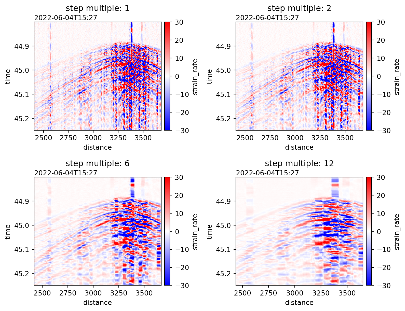
First, the smallest possible gauge length which occurs when step_multiple=1, in other words, the gauge length is equal to the distance step. For example, Figure 1 shows converting from velocity to strain rate for an event recorded by a Terra15 interrogator using function 2.

Code

import matplotlib.pyplot as plt

import dascore as dc

patch = dc.get_example_patch("deformation_rate_event_1")

fig, axes = plt.subplots(2, 2, figsize=(8.4, 6.5))

for sm, ax in zip([1, 2, 6, 12], axes.flatten()):
    # Convert to microstrain
    strain = (
        (patch.velocity_to_strain_rate_edgeless(step_multiple=sm) * 1e6)
        .update_attrs(data_units=None)
    )
    strain.viz.waterfall(ax=ax, scale=(-30, 30), scale_type="absolute")
    ax.set_title(f"step multiple: {sm}")

plt.tight_layout()
# plt.show()

Figure 1: Gauge length effects on event.

Notice how the noisy channels around distance 2600m and 3400m have lower amplitude but occur along more channels when the step_multiple is increased.

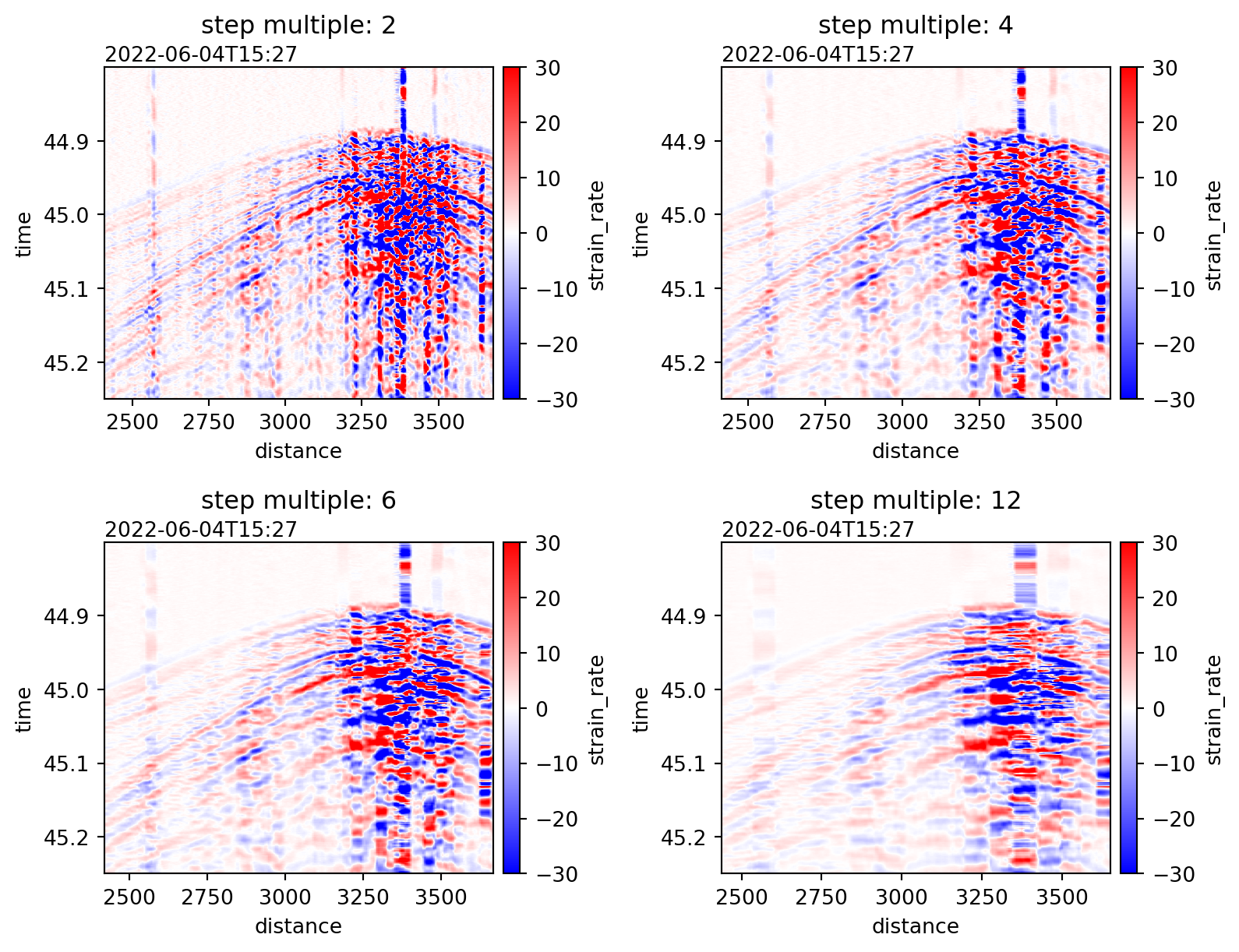
Using the first function, the smallest step_multiple is 2. Despite treating the edges differently, the outputs of function 2 are nearly tha same as function 1 and no significant edge effects are observable.

Code

import matplotlib.pyplot as plt

import dascore as dc

patch = dc.get_example_patch("deformation_rate_event_1")

fig, axes = plt.subplots(2, 2, figsize=(8.4, 6.5))

for sm, ax in zip([2, 4, 6, 12], axes.flatten()):
    # Convert to microstrain
    strain = (
        (patch.velocity_to_strain_rate_edgeless(step_multiple=sm) * 1e6)
        .update_attrs(data_units=None)
    )
    strain.viz.waterfall(ax=ax, scale=(-30, 30), scale_type="absolute")
    ax.set_title(f"step multiple: {sm}")

plt.tight_layout()
# plt.show()

Figure 2: Gauge length effects on event.

Higher order filters

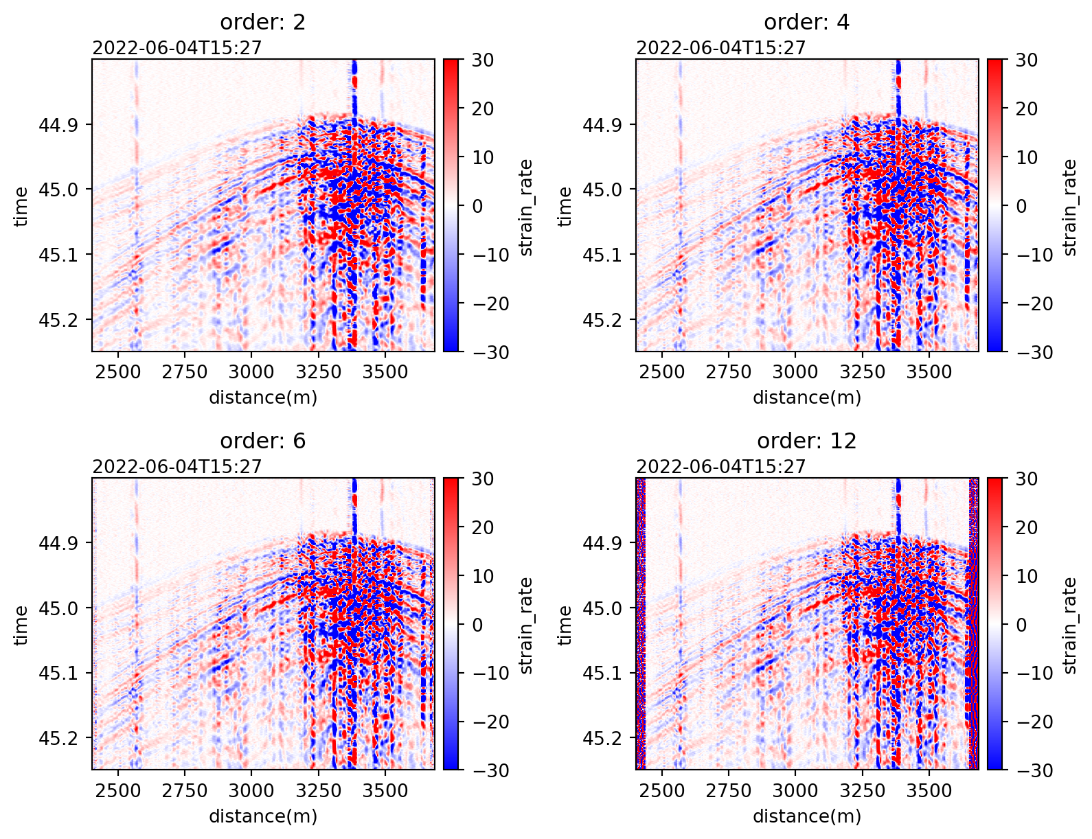
Rather than simple finite differences using only two points, higher order filters are possible with deformation rate data. Yang, Shragge, and Jin (2022) discuss the advantages of such an approach. Figure 3 shows the same event from above with different orders applied.

Code

import matplotlib.pyplot as plt

import dascore as dc

patch = dc.get_example_patch("deformation_rate_event_1")

fig, axes = plt.subplots(2, 2, figsize=(8.4, 6.5))

for order, ax in zip([2, 4, 6, 12], axes.flatten()):
    # Convert to microstrain
    strain = (
        (patch.velocity_to_strain_rate(order=order) * 1e6)
        .update_attrs(data_units=None)
    )
    strain.viz.waterfall(ax=ax, scale=(-30, 30), scale_type="absolute")
    ax.set_title(f"order: {order}")

plt.tight_layout()

Warning

Notice in Figure 3 some significant filter artefacts along the edge channels are introduced for the higher order filters.

References

Yang, Jihyun, Jeffrey Shragge, and Ge Jin. 2022. “Filtering Strategies for Deformation-Rate Distributed Acoustic Sensing.” Sensors 22 (22): 8777.