F-K Transform and Filtering

FK transforms

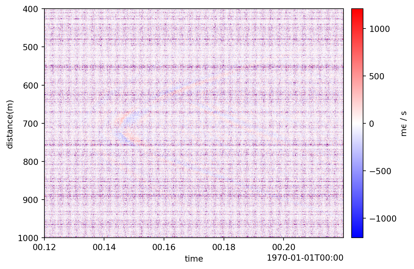
F-k transforms are common in geophysical applications for various types of filtering. For the following examples we will use the example_event included in DASCore’s example files.

import numpy as np
import matplotlib.pyplot as plt

import dascore as dc

patch = (
    dc.get_example_patch('example_event_1')
    .set_units("mstrain/s", distance='m', time='s')
)

patch.viz.waterfall(scale=0.2);

With some simple processing, as shown in other parts of the tutorial, we can clean up the patch:

import dascore as dc

patch_filtered = (
    patch.taper(time=0.075)
    .pass_filter(time=(None, 300))
)

patch_filtered.viz.waterfall(show=True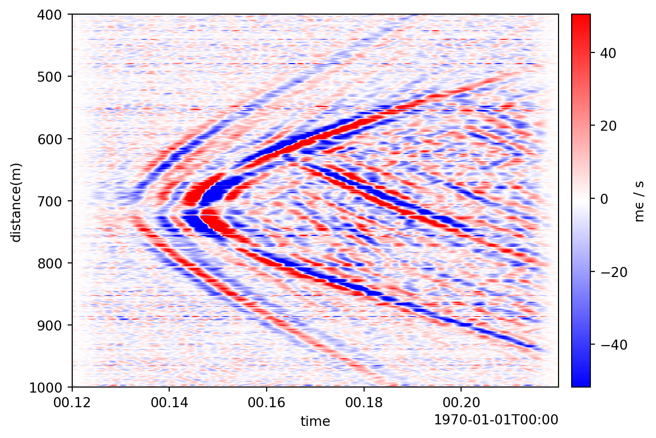, scale=0.2);

We can transform and visualize the patch in the F-K domain using the dft.

# Apply transform on all dimensions
fk_patch = patch_filtered.dft(patch.dims)

# We can't plot complex arrays so only plot amplitude
ax = fk_patch.abs().viz.waterfall()

# Zoom in around interesting frequencies
ax.set_xlim(-500, 500);
ax.set_ylim(-.2, .2);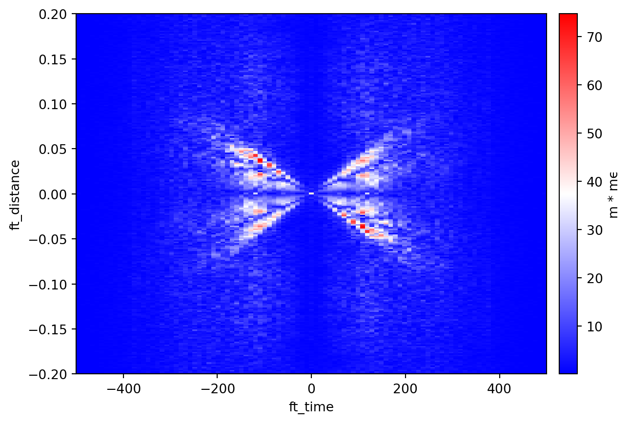

Slope Filtering

One advantage of the FK transform is the ability to manipulate signals based on their apparent velocities. Patch.slope_filter can be used for this purpose.

For example, given the first example event, we can apply a slope filter whose range covers reasonable seismic velocities. The filt parameter specifies the slope (apparent velocities). It is a 4 length sequence of the form [va, vb, vc, vd] where velocities between vb and vc are unchanged (or set to zero if the notch parameter is True) and values between va and vb, as well as those between vc and vd, are tapered.

filt = np.array([2_000, 2_200, 8_000, 9_000])
patch_filtered_2 = patch_filtered.slope_filter(filt=filt)
patch_filtered_2.viz.waterfall(scale=1);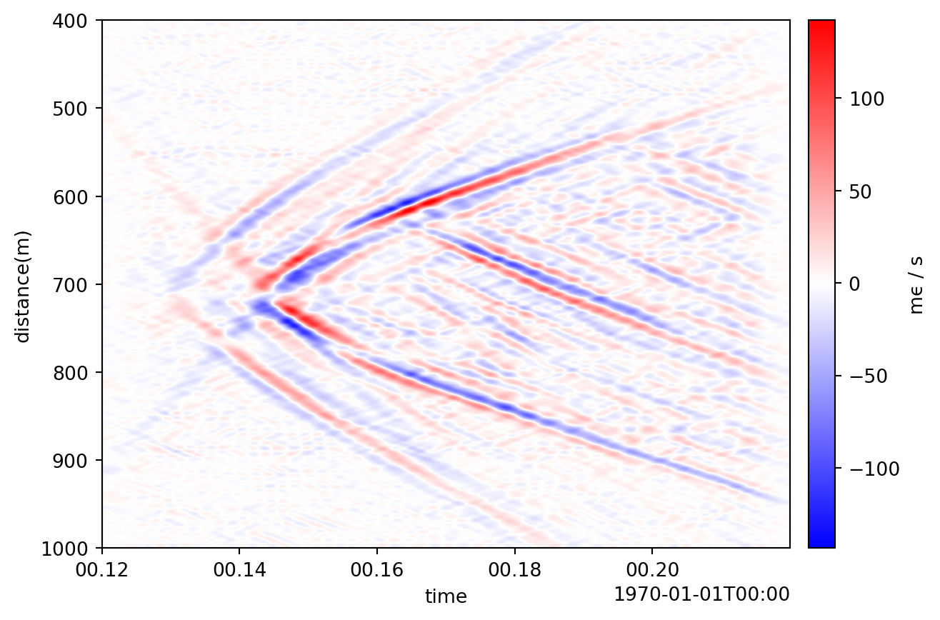

Note

It’s important to remember that apparent velocities (>= velocity) are filtered. For the case of local seismicity occurring near the cable the apparent velocity will approximate the medium velocity for part of the recording. Additional considerations are needed for more distant events.

Phase Separation

Another application of slope_filter is to separate P/S waves. In this case, the P velocity is about 4500 amd the S velocity is about 2700. The following code highlights S waves, but also introduces some artifacts:

filt_p = np.array([1_000, 2_300, 3_000, 4_000])
patch_filtered_p = patch_filtered.slope_filter(filt=filt_p)
patch_filtered_p.viz.waterfall(scale=1);

Up/Down separation

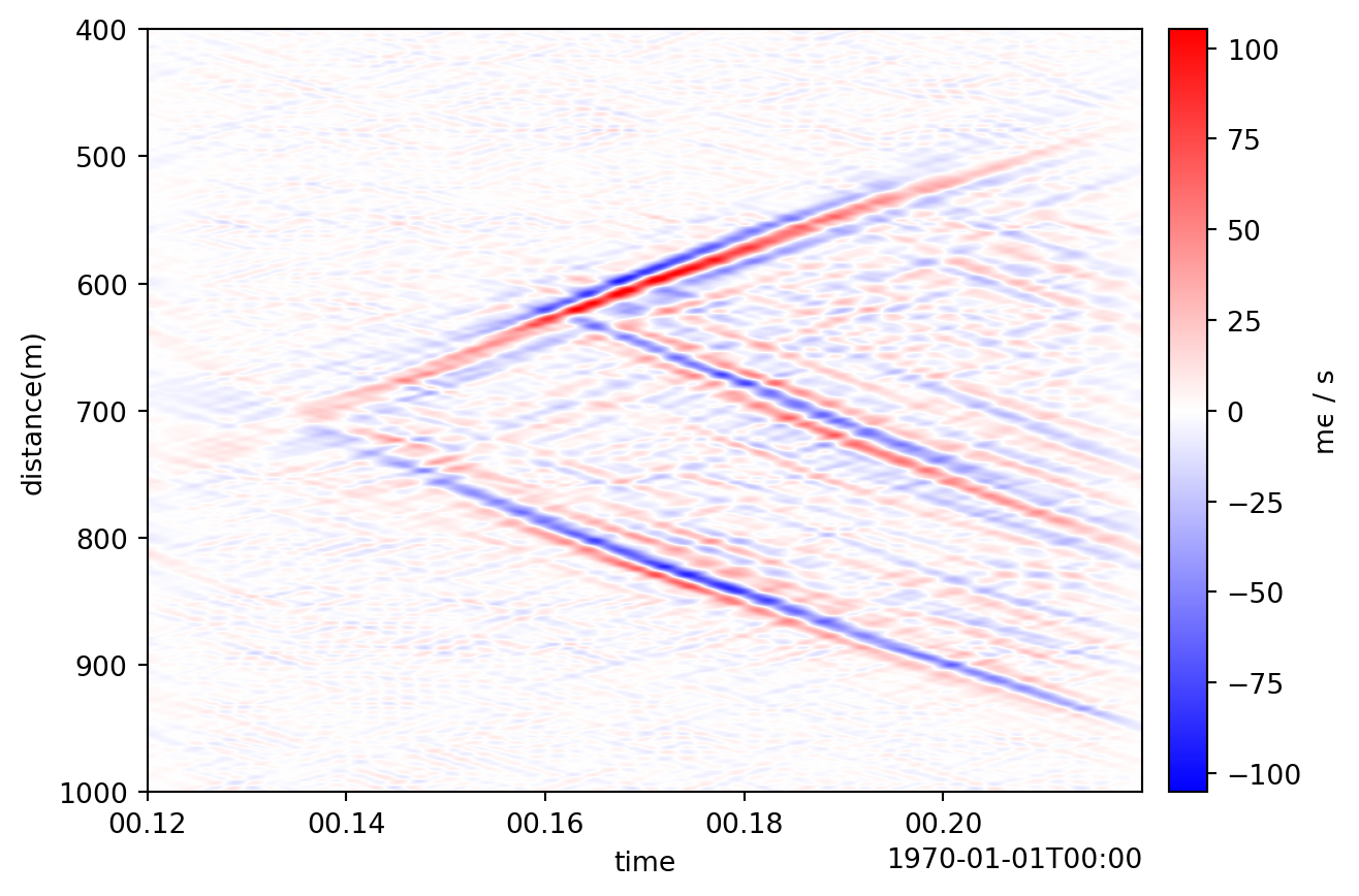
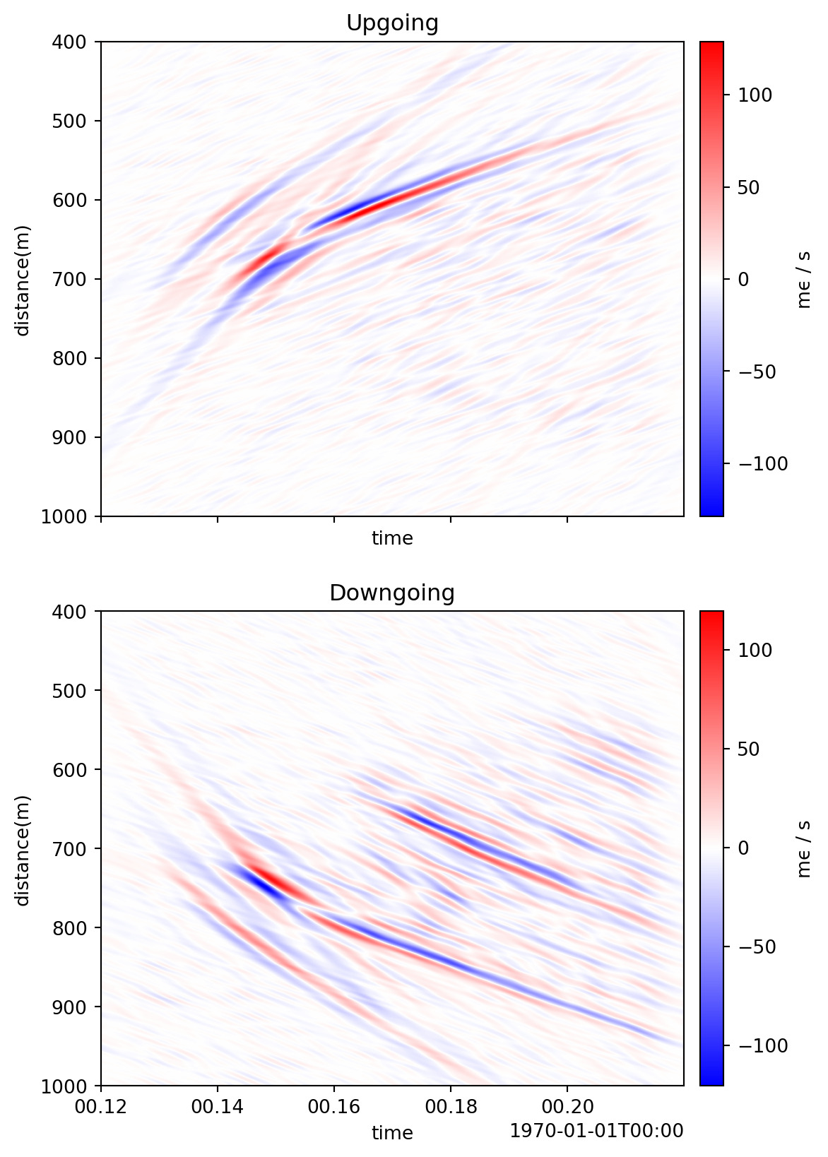
Up/down (or left/right) separation is also possible using the directional keyword. Up-going (waves moving towards the interrogator according a decreasing distance value) have positive velocities and down-going (waves moving away from the interrogator) have negative velocities.

patch_upgoing = patch_filtered.slope_filter(filt=filt, directional=True)
patch_downgoing = patch_filtered.slope_filter(filt=-filt[::-1], directional=True)

fig, (ax_up, ax_down) = plt.subplots(2, 1, figsize=(6,10), sharex=True)

patch_upgoing.viz.waterfall(scale=1, ax=ax_up);
ax_up.set_title("Upgoing");
patch_downgoing.viz.waterfall(scale=1, ax=ax_down);
ax_down.set_title("Downgoing");