import numpy as np
import matplotlib.pyplot as plt

import dascore as dc

patch = (
    dc.get_example_patch('example_event_1')
    .set_units("mstrain/s", distance='m', time='s')
)

patch.viz.waterfall();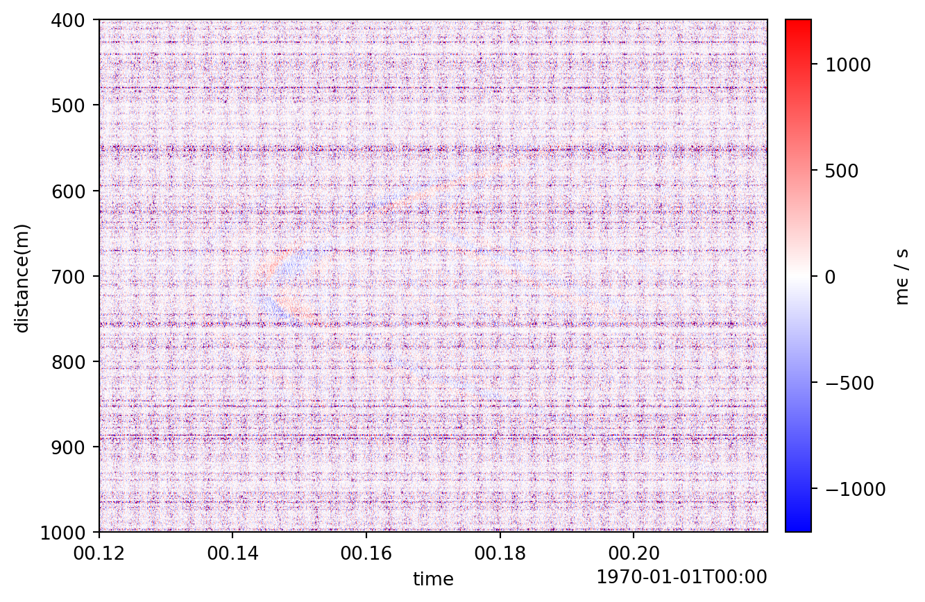
Use an F-K transform to filter by frequency and apparent velocity.
import numpy as np
import matplotlib.pyplot as plt
import dascore as dc
patch = (
dc.get_example_patch('example_event_1')
.set_units("mstrain/s", distance='m', time='s')
)
patch.viz.waterfall();
Taper and band-pass before transforming:
import dascore as dc

patch_filtered = (
    patch.taper(time=0.075)
    .pass_filter(time=(None, 300))
)

patch_filtered.viz.waterfall(show=True);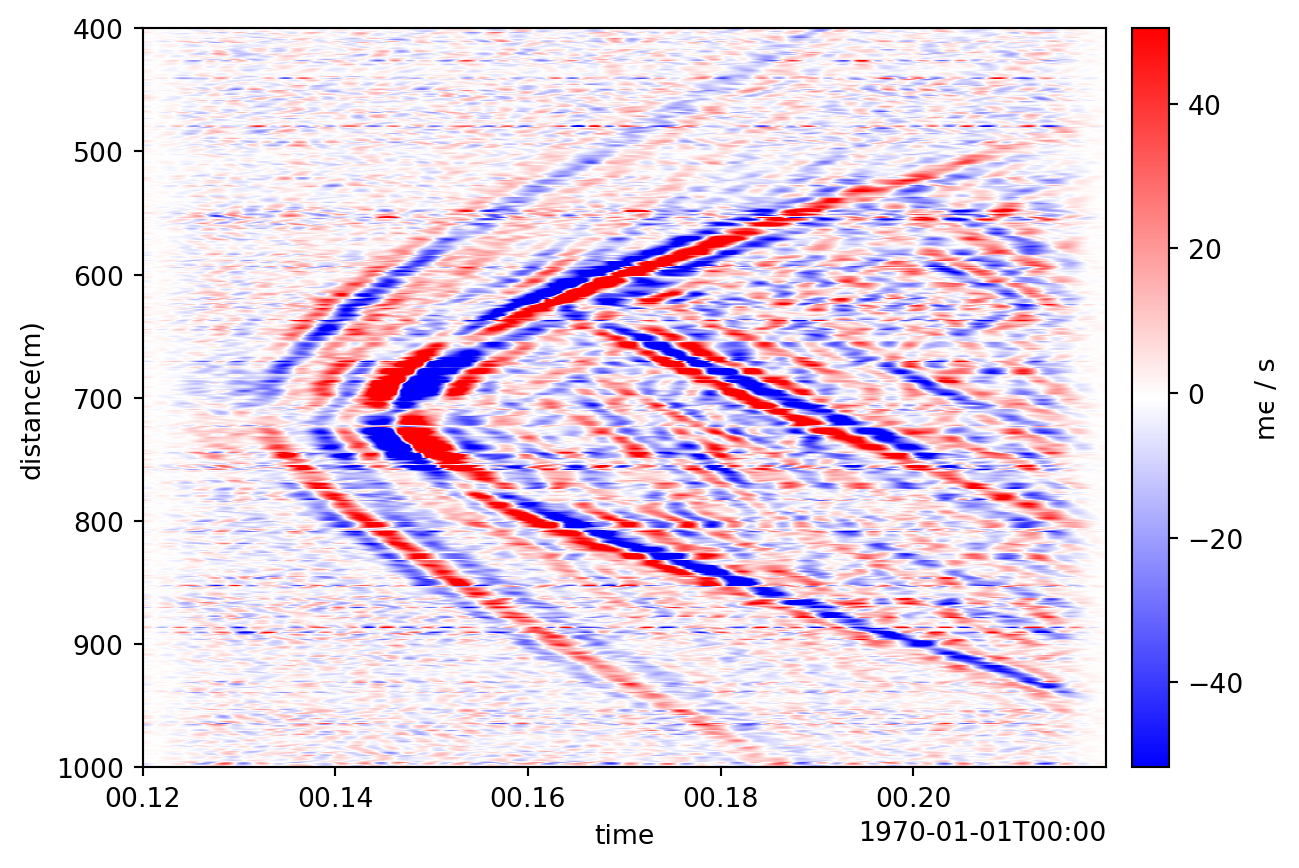
Transform both dimensions and plot amplitude because the DFT is complex:
fk_patch = patch_filtered.dft(patch.dims)
ax = fk_patch.abs().viz.waterfall()
ax.set_xlim(-500, 500);
ax.set_ylim(-.2, .2);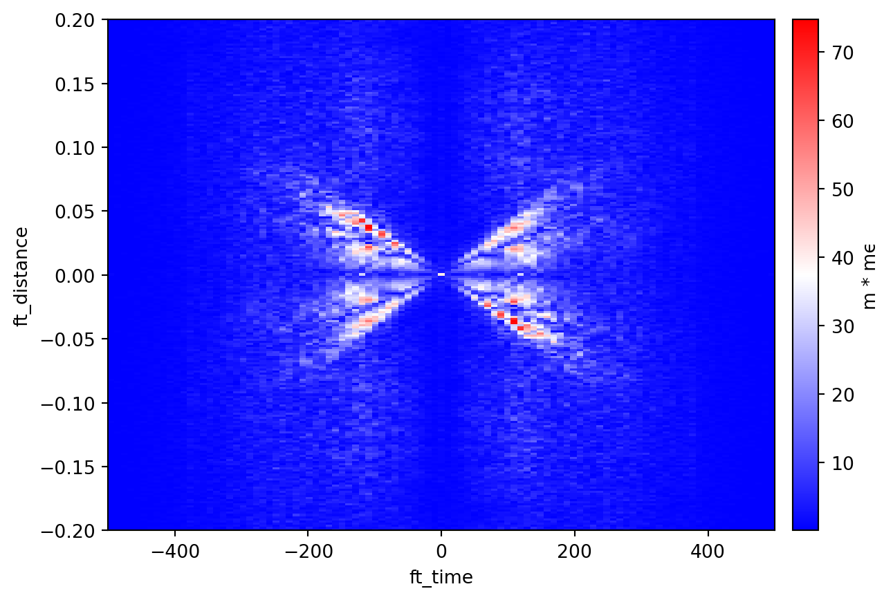
Patch.slope_filter takes [va, vb, vc, vd]: values between vb and vc pass (or are removed with invert=True), and the outer intervals taper.
filt = np.array([2_000, 2_200, 8_000, 9_000])
patch_filtered_2 = patch_filtered.slope_filter(filt=filt)
patch_filtered_2.viz.waterfall(scale=1);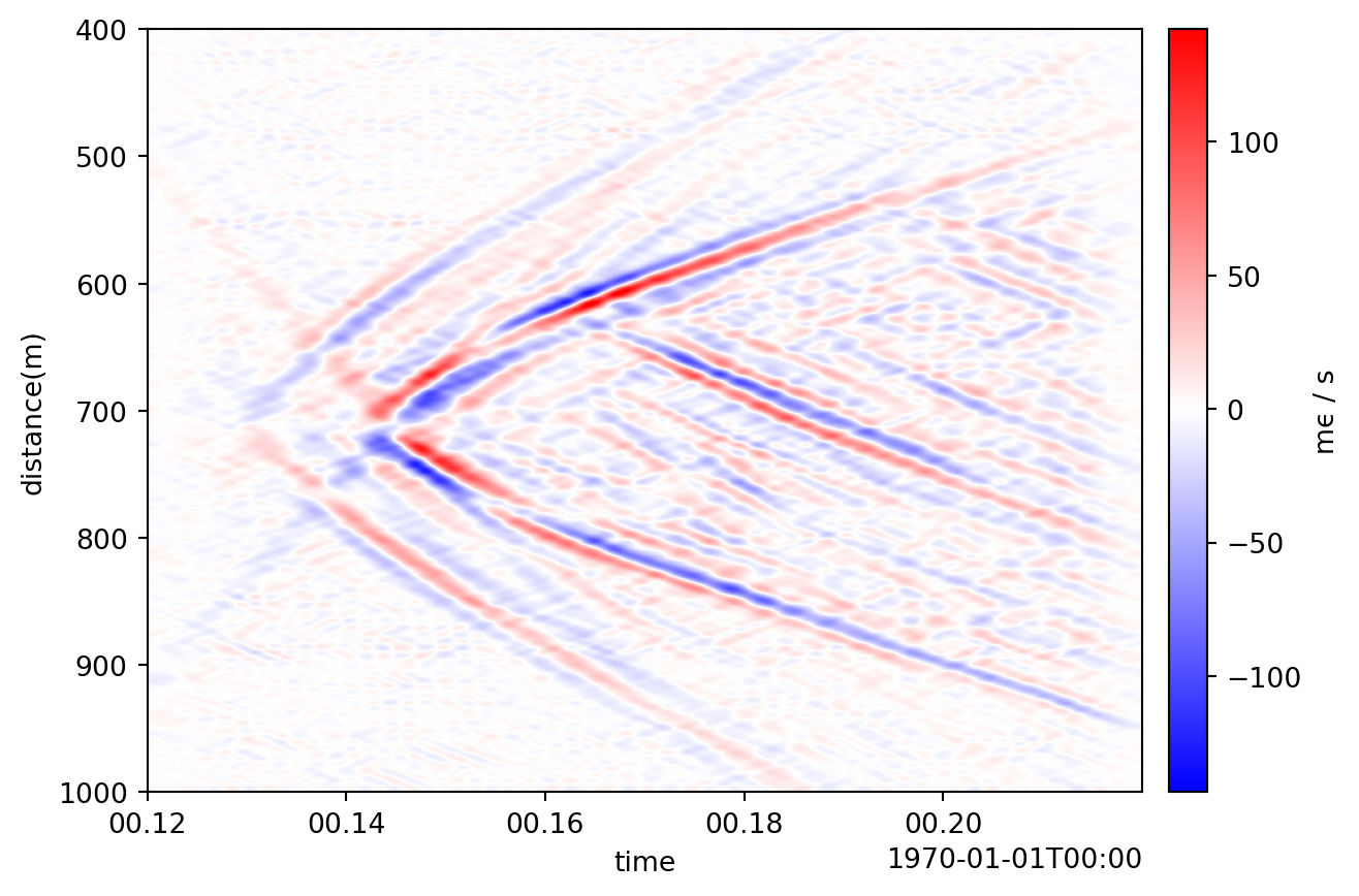
The filter uses apparent velocity. It approximates medium velocity only for suitable local geometry.
This range highlights an S wave near 2700 m/s while rejecting a P wave near 4500 m/s:
filt_s = np.array([1_000, 2_300, 3_000, 4_000])
patch_filtered_s = patch_filtered.slope_filter(filt=filt_s)
patch_filtered_s.viz.waterfall(scale=1);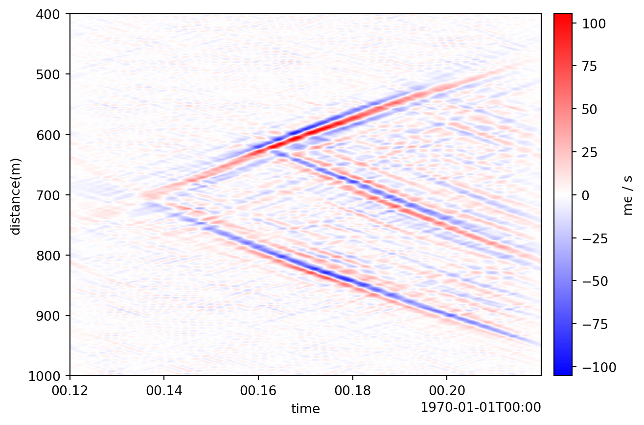
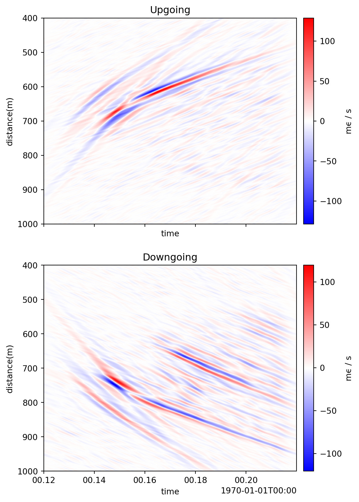
On a near-linear fiber, directional=True separates positive velocities moving toward decreasing distance from negative velocities moving toward increasing distance.
patch_upgoing = patch_filtered.slope_filter(filt=filt, directional=True)
patch_downgoing = patch_filtered.slope_filter(filt=-filt[::-1], directional=True)

fig, (ax_up, ax_down) = plt.subplots(2, 1, figsize=(6,10), sharex=True)

patch_upgoing.viz.waterfall(scale=1, ax=ax_up);
ax_up.set_title("Upgoing");
patch_downgoing.viz.waterfall(scale=1, ax=ax_down);
ax_down.set_title("Downgoing");