Low-Frequency Processing

This recipe demonstrates how DASCore can be used to apply low-frequency (LF) processing to a spool of DAS data. LF processing helps efficiently downsample the entire spool.

Get a spool and define parameters

import tempfile
from pathlib import Path

import numpy as np
import os

import dascore as dc
from dascore.utils.patch import get_patch_names

## Load libraries and get a spool to work on
# Define path for saving results (swap out with your path)
output_data_dir = Path(tempfile.mkdtemp())

# Get a spool to work on
sp = dc.get_example_spool().update()

# Sort the spool
sp = sp.sort("time")
# You may also want to sub-select the spool for the desired distance or time samples before proceeding.

# Get the first patch
pa = sp[0]

# Define the target sampling interval (in sec.)
dt = 1
# With a sampling interval of 10 seconds, the cutoff frequency (Nyquist frequency) is determined to be 0.05 Hz 
cutoff_freq = 1 / (2*dt)

# Safety factor for the low-pass filter to avoid ailiasing 
filter_safety_factor = 0.9

# Enter memory size to be dedicated for processing (in MB)
memory_limit_MB = 1_000

# Define a tolerance for determining edge effects (used in next step)
tolerance = 1e-3

Calculate chunk size and determine edge effects

To chunk the spool, first we need to figure out the chunk size based on machine’s memory size so we ensure we can load and process patches with no memory issues. Longer chunk size (longer patches) increases computation efficiency.

Notes:

The processing_factor is required because certain processing routines involve making copies of the data during the processing steps. It should be determined by performing memory profiling on an example dataset for the specific processing routine. For instance, the combination of low-pass filtering and interpolation, discussed in the next section, requires a processing factor of approximately 5.
The memory_safety_factor is optional and helps prevent getting too close to the memory limit.

# Get patch's number of bytes per seconds (based on patch's data type) 
pa_bytes_per_second = pa.data.nbytes / pa.seconds
# Define processing factor and safety factor 
processing_factor = 5  
memory_safety_factor = 1.2 

# Calculate memory size required for each second of data to get processed
memory_size_per_second = pa_bytes_per_second * processing_factor * memory_safety_factor
memory_size_per_second_MB = memory_size_per_second / 1e6

# Calculate chunk size that can be loaded (in seconds)
chunk_size = memory_limit_MB / memory_size_per_second_MB

# Ensure `chunk_size` does not exceed the spool length
time_step = sp[0].get_coord('time').step
time_min = sp[0].get_coord('time').min()
time_max = sp[-1].get_coord('time').max()
spool_length = dc.to_float((time_max - time_min + time_step))
if chunk_size > spool_length:
   print(
   f"Warning: Specified `chunk_size` ({chunk_size:.2f} seconds) exceeds the spool length "
   f"({spool_length:.2f} seconds). Adjusting `chunk_size` to match spool length."
   )
   chunk_size = spool_length

Warning: Specified `chunk_size` (277.78 seconds) exceeds the spool length (24.00 seconds). Adjusting `chunk_size` to match spool length.

Next, we need to determine the extent of artifacts introduced by low-pass filtering at the edges of each patch. To achieve this, we apply LF processing to a delta function patch, which contains a unit value at the center and zeros elsewhere. The distorted edges are then identified based on a defined threshold.

# Retrieve a patch of appropriate size for LF processing that fits into memory
pa_chunked_sp = sp.chunk(time=chunk_size, keep_partial=True)[0] 
# Create a delta patch based on new patch size
delta_pa = dc.get_example_patch("delta_patch", dim="time", patch=pa_chunked_sp)

# Apply the low-pass filter on the delta patch
delta_pa_low_passed = delta_pa.pass_filter(time=(None, cutoff_freq * filter_safety_factor))
# Resample the low-passed filtered patch
new_time_ax = np.arange(delta_pa.attrs["time_min"], delta_pa.attrs["time_max"], np.timedelta64(dt, "s"))
delta_pa_lfp = delta_pa_low_passed.interpolate(time=new_time_ax)

# Identify the indices where the absolute value of the data exceeds the threshold
data_abs = np.abs(delta_pa_lfp.data)
threshold = np.max(data_abs) * tolerance
ind = data_abs > threshold
ind_1 = np.where(ind)[1][0]
ind_2 = np.where(ind)[1][-1]

# Get the total duration of the processed delta function patch in seconds
delta_pa_lfp_length = delta_pa_lfp.seconds 
# Convert the new time axis to absolute seconds, relative to the first timestamp
time_ax_abs = (new_time_ax - new_time_ax[0]) / np.timedelta64(1, "s")
# Center the time axis 
time_ax_centered = time_ax_abs - delta_pa_lfp_length // 2 

# Calculate the maximum of edges in both sides (in seconds) where artifacts are present
edge = max(np.abs(time_ax_centered[ind_1]), np.abs(time_ax_centered[ind_2]))

# Validate the `edge` value to ensure sufficient processing patch size
if np.ceil(edge) >= chunk_size / 2:
    raise ValueError(
        f"The calculated `edge` value ({edge:.2f} seconds) is greater than half of the processing patch size "
        f"({chunk_size:.2f} seconds). To resolve this and increase efficiency, consider one of the following:\n"
        "- Increase `memory_size` to allow for a larger processing window.\n"
        "- Increase `tolerance` to reduce the sensitivity of artifact detection."
    )

Perform low-frequency processing and save results on disk

# First we chunk the spool based on the `chunk_size' and `edge` calculated before.
sp_chunked_overlap = sp.chunk(time=chunk_size, overlap=2*edge, keep_partial=True)

# Process each patch in the spool and save the result patch
lf_patches = []
for patch in sp_chunked_overlap:
    # Apply any pre-processing you may need (such as velocity to strain rate transformation, detrending, etc.)
    # ...

    # Apply the low-pass filter on the delta patch
    pa_low_passed = patch.pass_filter(time=(..., cutoff_freq * filter_safety_factor))
    # Resample the low-passed filter patch
    new_time_ax = np.arange(pa_low_passed.attrs["time_min"], pa_low_passed.attrs["time_max"], np.timedelta64(dt, "s"))
    pa_lfp = (
        pa_low_passed.interpolate(time=new_time_ax)
        .update_coords(time_step=dt)   # Update sampling interval
        # remove edges from data at both ends
        .select(time=(edge, -edge), relative=True)
    )
    
    # Save processed patch 
    pa_lf_name = pa_lfp.get_patch_name()
    path = output_data_dir / f"{pa_lf_name}.h5"
    pa_lfp.io.write(path, "dasdae")

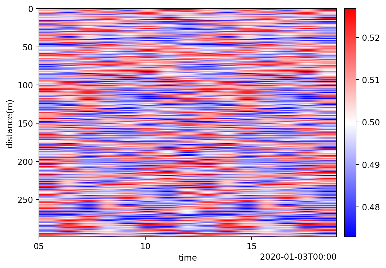
Visualize the results

# Create a spool of LF processed results
sp_lf = dc.spool(output_data_dir) 

# Merge the spool and create a single patch. May need to sub-select before merging to prevent exceeding the memory limit.
sp_lf_merged = sp_lf.chunk(time=None, conflict="keep_first")
pa_lf_merged = sp_lf_merged[0]

# Visualize the results. Try different scale values for better Visualization.
pa_lf_merged.viz.waterfall(scale=0.5)

<Axes: xlabel='time', ylabel='distance(m)'>

For any questions, please contact Ahmad Tourei.