import io
import tempfile
from pathlib import Path

import numpy as np
import pandas as pd

import dascore as dc
from dascore.examples import tunnel_inventory_files, write_tunnel_inventory

files = tunnel_inventory_files(repaired=False)
root = Path(tempfile.mkdtemp()) / "tunnel_inventory"
write_tunnel_inventory(root, repaired=False)


def show(name):
    """Print one of the inventory's files."""
    print(files[name])


def table(name):
    """Read one of the inventory's CSV files back as a frame."""
    return pd.read_csv(io.StringIO(files[name]))


PATH = "fiber_arrays/XT.TUN1/path.00"Create an inventory
Create, validate, repair, serialize, and attach an inventory using a worked tunnel deployment.
Keywords
inventory, geometry, deployment, validation
Use an inventory to describe the observing system independently of the files containing its measurements. Start from recorded deployment facts; the tunnel example below shows how the pieces fit together.
Workflow
- Gather known identity, resource, survey, coupling, acquisition, and validity-time information. Keep unknown deployment facts explicit. Do not invent serial numbers, coordinates, dates, or installation details to fill a schema.
- Separate owned resources from components on the optical path, geometry, coupling, labels, and acquisition configuration. Model a continuous run with a shared break history as one fiber array and path.
- Use the installed schema’s canonical attributes and declared units. Distinguish instrument distance, optical distance, and survey coordinates, including their reference frame. Represent winding and other geometry through coordinate mappings rather than ad hoc corrections.
- Load the authored description with
dc.inventory(...)to validate schemas, references, and track bounds. Repair source mistakes using evidence; represent a changed deployment with a new dated epoch rather than overwriting its history. - Serialize with
inventory.io.to_yaml(), reload withdc.inventory(text), and compare the result. The final example below performs this round trip. - Attach the inventory to a small representative spool with matching acquisition keys and recording times. Check selected regions and enriched coordinates, including unknown positions. Test epoch boundaries when configuration or geometry changes during the data.
Consult python -m dascore doc Inventory with the selected environment’s Python executable, and read the relevant field or method documentation when adapting the example to a different deployment.
Tunnel example
This end-to-end inventory example models an underground tunnel deployment from survey files through enriched patches. A 1500 m telemetry cable feeds trenched fiber, a buried coil, and three instrumented boreholes.
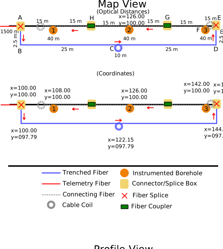
Hardware uses YAML files; tabular tracks use CSV. All example files are bundled with DASCore.
What the drawing says
Reading Figure 1 along the fiber, from the interrogator:
| From | To | What the light passes through | Optical |
|---|---|---|---|
| instrument room | A | telemetry cable | 1500 m |
| A | B | drop into the trench | 2.5 m |
| B | C | trenched sensing fiber | 25 m |
| C | the buried coil | 10 m | |
| C | D | trenched sensing fiber | 25 m |
| D | E | rise out of the trench | 2.5 m |
| E | 3, 2, 1 | six links between splice boxes, couplers, and borehole heads | 15 m each |
| three boreholes, down and back | 40 m each |
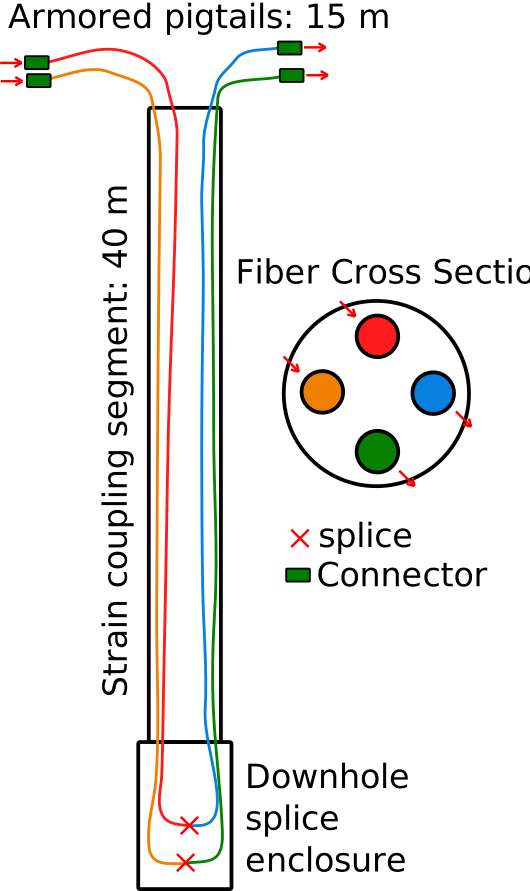
A 20 m borehole holds 40 m of sensing fiber because the cable returns to the surface.
The trenched cable is wound helically, so ground distance \(d_r\) is shorter than optical distance \(d_o\):
\[ d_r \approx d_o \cos \phi \approx 0.886\, d_o \]
Thus 25 m of fiber covers 22.15 m of tunnel. The geometry track stores this mapping so consumers use coordinates directly.
The hardware
Cables, enclosures, and interrogators live under resources/; filenames become referenced resource_id values.
resources/*.yaml — the hardware, from the purchase orders
for name in sorted(x for x in files if x.startswith("resources/")):
    print(f"# {name}")
    print(files[name])
# resources/borehole-cable.yaml
object_type: Cable
name: borehole sensing cable
manufacturer: Nerve Sensors
model: Epsilon
fiber_count: 4
description: Rock-coupled downhole cable with an armored pigtail.
# resources/connecting-cable.yaml
object_type: Cable
name: tunnel connecting cable
manufacturer: Corning
model: MIC tight-buffered 4F OS2
fiber_count: 4
description: The links between boxes, couplers, and borehole heads.
# resources/das-interrogator.yaml
object_type: Interrogator
name: tunnel DAS interrogator
manufacturer: Sintela
model: Onyxia
instrument_type: DAS interrogator
# resources/splice-box-a.yaml
object_type: Enclosure
name: tunnel splice box at A
enclosure_type: box
# resources/splice-box-e.yaml
object_type: Enclosure
name: tunnel splice box at E
enclosure_type: box
# resources/telemetry-cable.yaml
object_type: Cable
name: tunnel telemetry cable
manufacturer: Corning
model: MIC tight-buffered 4F OS2
fiber_count: 4
description: The run in from the instrument room.
# resources/trench-cable.yaml
object_type: Cable
name: helically wound trench cable
manufacturer: Silixa
model: HWC
fiber_count: 1
# resources/turnaround-1.yaml
object_type: Enclosure
name: tunnel borehole 1 turnaround housing
enclosure_type: housing
# resources/turnaround-2.yaml
object_type: Enclosure
name: tunnel borehole 2 turnaround housing
enclosure_type: housing
# resources/turnaround-3.yaml
object_type: Enclosure
name: tunnel borehole 3 turnaround housing
enclosure_type: housing
The inventory envelope defines a local x, y, z survey grid in meters, with z positive upward.
show("inventory.yaml")
show("fiber_arrays/XT.TUN1/attrs.yaml")
object_type: Inventory
coordinate_reference_system:
authority: local
code: tunnel
name: tunnel engineering grid
coordinate_labels: [x, y, z]
units: [meter, meter, meter]
object_type: FiberArray
name: tunnel fiber array
The path, as a table
Optical components tile the path with distance_min and distance_max. Point components such as splices state one distance. Location code 00 names the path.00 directory.
path.00/optical_components.csv
components_csv = files[f"{PATH}/optical_components.csv"]

table(f"{PATH}/optical_components.csv").head(9)| object_type | distance_min | distance_max | name | container | |
|---|---|---|---|---|---|
| 0 | FiberSegment | 0.0 | 1500.0 | telemetry lead-in | telemetry-cable |
| 1 | Splice | 1500.0 | NaN | splice at box A | splice-box-a |
| 2 | FiberSegment | 1500.0 | 1502.5 | drop into the trench | trench-cable |
| 3 | FiberSegment | 1502.5 | 1527.5 | trench B to the coil | trench-cable |
| 4 | FiberSegment | 1527.5 | 1537.5 | cable coil at C | trench-cable |
| 5 | FiberSegment | 1537.5 | 1562.5 | trench from the coil to D | trench-cable |
| 6 | FiberSegment | 1562.5 | 1565.0 | rise out of the trench | trench-cable |
| 7 | Splice | 1565.0 | NaN | splice at box E | splice-box-e |
| 8 | FiberSegment | 1565.0 | 1580.0 | link E to borehole 3 | connecting-cable |
object_type selects the row model, distances determine order, and container values reference resources. Other tracks use the same optical distances:
def spans(csv_text):
    """Map each component's name to the optical interval it covers."""
    frame = pd.read_csv(io.StringIO(csv_text))
    # A point component states one distance; the other end is the same one.
    ends = frame["distance_max"].fillna(frame["distance_min"])
    return dict(zip(frame["name"], zip(frame["distance_min"], ends)))


at = spans(components_csv)

print("borehole 3 sensing fiber:", at["borehole 3 down"][0], "to", at["borehole 3 up"][1])
borehole 3 sensing fiber: 1580.0 to 1620.0Where the fiber is
Geometry pairs surveyed control points with the fiber segments between them.
path.00/geometry.csv — the survey points, paired with the fiber between them
geometry = table(f"{PATH}/geometry.csv")

geometry.head(8)| name | distance | x | y | z | |
|---|---|---|---|---|---|
| 0 | drop into the trench | 1500.0 | 100.00 | 100.00 | 0.0 |
| 1 | drop into the trench | 1502.5 | 100.00 | 97.79 | -0.5 |
| 2 | trench B to the coil | 1502.5 | 100.00 | 97.79 | -0.5 |
| 3 | trench B to the coil | 1527.5 | 122.15 | 97.79 | -0.5 |
| 4 | trench from the coil to D | 1537.5 | 122.15 | 97.79 | -0.5 |
| 5 | trench from the coil to D | 1562.5 | 144.30 | 97.79 | -0.5 |
| 6 | rise out of the trench | 1562.5 | 144.30 | 97.79 | -0.5 |
| 7 | rise out of the trench | 1565.0 | 144.30 | 100.00 | 0.0 |
Unsurveyed slack links and the coil remain nan rather than receiving invented positions. Control-point interpolation captures the helical mapping without storing a wind angle.
How it is attached to the ground
Coupling is interval metadata: coupling_type is controlled, while medium and attachment add detail.
path.00/coupling.csv
coupling = table(f"{PATH}/coupling.csv")

coupling| distance_min | distance_max | coupling_type | medium | attachment | depth | |
|---|---|---|---|---|---|---|
| 0 | 1500.0 | 1502.5 | trench | soil | direct_burial | 0.5 |
| 1 | 1502.5 | 1527.5 | trench | soil | direct_burial | 0.5 |
| 2 | 1537.5 | 1562.5 | trench | soil | direct_burial | 0.5 |
| 3 | 1562.5 | 1565.0 | trench | soil | direct_burial | 0.5 |
| 4 | 1527.5 | 1537.5 | coiled | soil | NaN | 0.5 |
| 5 | 1580.0 | 1620.0 | outside_borehole_casing | rock | cemented | NaN |
| 6 | 1650.0 | 1690.0 | outside_borehole_casing | rock | cemented | NaN |
| 7 | 1720.0 | 1760.0 | outside_borehole_casing | rock | cemented | NaN |
The coil is coiled, not trench, because it does not sample a unique position.
Everything else
Labels become selectable patch coordinates. Here section identifies installation type and borehole numbers the holes.
path.00/labels.csv
labels = table(f"{PATH}/labels.csv")

labels| distance_min | distance_max | group | value | |
|---|---|---|---|---|
| 0 | 1500.0 | 1502.5 | section | trench |
| 1 | 1502.5 | 1527.5 | section | trench |
| 2 | 1537.5 | 1562.5 | section | trench |
| 3 | 1562.5 | 1565.0 | section | trench |
| 4 | 1527.5 | 1537.5 | section | coil |
| 5 | 1580.0 | 1620.0 | section | borehole |
| 6 | 1580.0 | 1620.0 | borehole | 3 |
| 7 | 1650.0 | 1690.0 | section | borehole |
| 8 | 1650.0 | 1690.0 | borehole | 2 |
| 9 | 1720.0 | 1760.0 | section | borehole |
| 10 | 1720.0 | 1760.0 | borehole | 1 |
Each label group must use one value type.
How the instrument was set up
An acquisition describes an instrument configuration on the path. Its filename yields acquisition key XT.TUN1.00.DAS; distance_map maps instrument distance to optical distance and remains explicit even when it is the identity.
show("acquisitions/XT.TUN1.00.DAS.yaml")object_type: Acquisition
data_category: DAS
data_type: strain_rate
data_units: 1/s
interrogator: das-interrogator
gauge_length: 10.0
spatial_interval: 1.0
sample_rate: 250.0
distance_map:
instrument_distance: [0.0, 2000.0]
distance: [0.0, 2000.0]
Reading it back
Loading validates schemas, resource references, and track bounds.
inventory = dc.inventory(root)

path = inventory.networks[0].fiber_arrays[0].optical_paths[0]
print(f"{path.optical_length:.1f} m of fiber in {len(path.optical_components)} components")

names = inventory.get_names()
print("coords:", [x for x in names.coords if "." not in x])
1775.0 m of fiber in 26 components
coords: ['distance', 'x', 'y', 'z', 'optical_components', 'geometry', 'coupling', 'section', 'borehole']Seeing it
Plot tracks against optical distance:
inventory.viz.path(distance=(1495, 1780), show=True);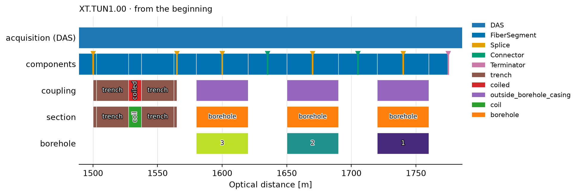
Or plot the local survey grid:
inventory.viz.map(x="x", y="z", color="section", show=True);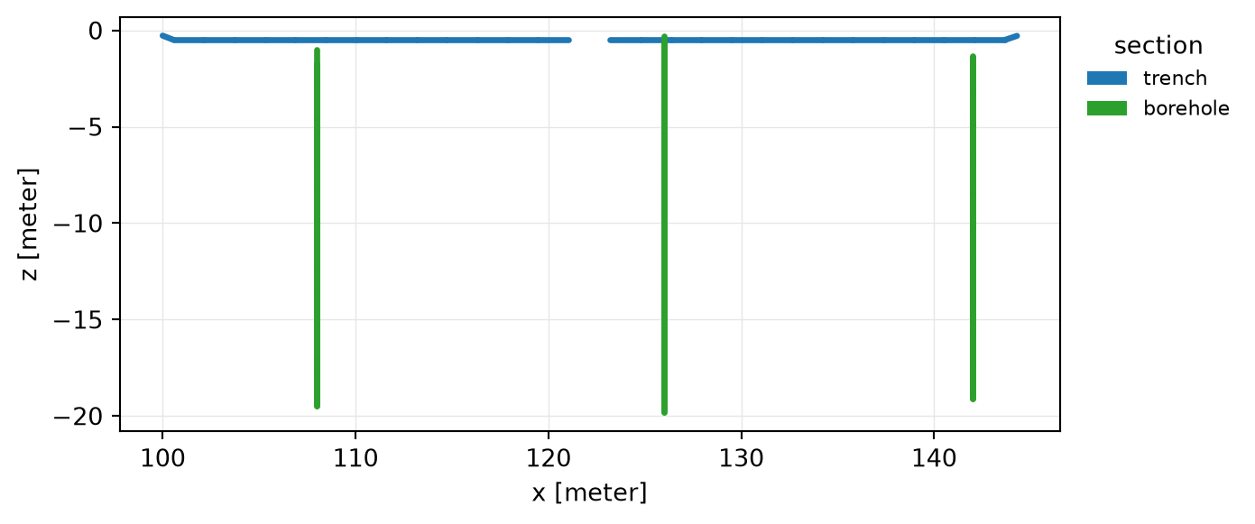
What the data gets out of it
A patch joins the inventory by acquisition key and time.
patch = dc.get_example_patch(
    "random_das",
    acquisition_key="XT.TUN1.00.DAS",
    time_min="2024-06-01",
    shape=(1776, 200),
)
spool = dc.spool(patch).attach_inventory(inventory)
Attaching reads no data; it makes inventory coordinates selectable:
boreholes = spool.select(section="borehole")

print(f"{len(boreholes)} runs of borehole fiber")
for sub in boreholes:
    distance = sub.get_coord("distance")
    print(f"  {distance.min()} to {distance.max()} m, {sub.shape[0]} channels")
3 runs of borehole fiber
1580 to 1620 m, 41 channels
1650 to 1690 m, 41 channels
1720 to 1760 m, 41 channelsThe three disjoint borehole runs return three patches.
Spool.enrich is what puts the metadata on a patch:
enriched = spool.enrich()[0]

print("gauge length:", enriched.attrs.gauge_length)
print("coordinates:", sorted(enriched.coords.coord_map))
gauge length: 10.0
coordinates: ['borehole', 'coupling', 'distance', 'section', 'time', 'x', 'y', 'z']Enrichment places surveyed channels and leaves unsurveyed ones unknown:
depth = enriched.get_coord("z").values
along = enriched.get_coord("x").values

assert depth[1590] == -10.0
assert np.isclose(along[1510], 100.0 + 7.5 * 0.886)
assert np.isnan(depth[1000])
A repair, and what it does to the data
In September, two splices and a two-meter patch cord repair a break 15 m into the trench. A new dated path epoch preserves the earlier geometry; its component table replaces one row with five and shifts downstream optical distances by two meters.
EPOCH = "fiber_arrays/XT.TUN1/path.00@2024-09-01"

files = tunnel_inventory_files(repaired=True)
write_tunnel_inventory(root, repaired=True)

repaired_components = table(f"{EPOCH}/optical_components.csv")
repaired_csv = files[f"{EPOCH}/optical_components.csv"]

index = int(repaired_components.index[repaired_components["name"] == "trench B to the break"][0])
repaired_components.iloc[index - 1 : index + 5]| object_type | distance_min | distance_max | name | container | |
|---|---|---|---|---|---|
| 2 | FiberSegment | 1500.0 | 1502.5 | drop into the trench | trench-cable |
| 3 | FiberSegment | 1502.5 | 1517.5 | trench B to the break | trench-cable |
| 4 | Splice | 1517.5 | NaN | repair splice near side | repair-box |
| 5 | FiberSegment | 1517.5 | 1519.5 | repair patch cord | repair-cord |
| 6 | Splice | 1519.5 | NaN | repair splice far side | repair-box |
| 7 | FiberSegment | 1519.5 | 1529.5 | trench from the break to the coil | trench-cable |
Generate all affected tracks from the repair description rather than editing distances independently.
path.00@2024-09-01 — the same tracks, against the new distances
repaired_at = spans(repaired_csv)

repaired_geometry = table(f"{EPOCH}/geometry.csv")
print(repaired_geometry.head(6).to_string(index=False))

repaired = dc.inventory(root)
for epoch in repaired.networks[0].fiber_arrays[0].optical_paths:
    began = "the beginning" if np.isnat(epoch.time_min) else str(epoch.time_min)[:10]
    print(f"from {began}: {epoch.optical_length:.1f} m")
name distance x y z
drop into the trench 1500.0 100.00 100.00 0.0
drop into the trench 1502.5 100.00 97.79 -0.5
trench B to the break 1502.5 100.00 97.79 -0.5
trench B to the break 1517.5 113.29 97.79 -0.5
trench from the break to the coil 1519.5 113.29 97.79 -0.5
trench from the break to the coil 1529.5 122.15 97.79 -0.5
from the beginning: 1775.0 m
from 2024-09-01: 1777.0 mPlot the epochs:
repaired.viz.timeline(show=True);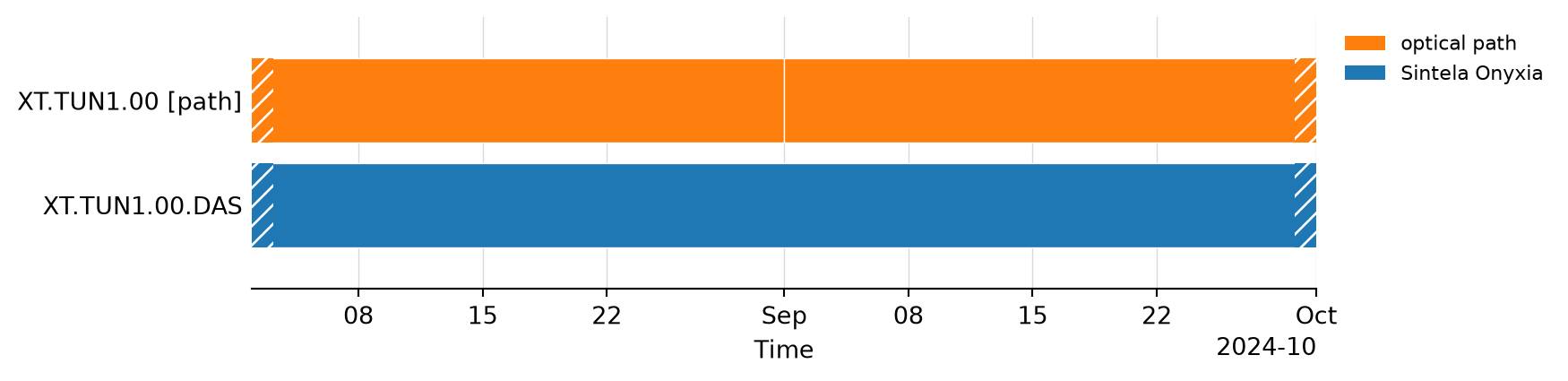
A patch spanning the epoch boundary matches both paths. Spool.conform_to_inventory splits it so each result has one valid description:
straddling = dc.get_example_patch(
    "random_das",
    acquisition_key="XT.TUN1.00.DAS",
    time_min="2024-08-31T23:59:59",
    shape=(1776, 500),
)
crossed = dc.spool(straddling).attach_inventory(repaired)

print("patches before:", len(crossed))
conformed = crossed.conform_to_inventory()
print("patches after: ", len(conformed))
print(conformed.get_contents()[["time_min", "time_max"]].to_string(index=False))
patches before: 1
patches after: 2
time_min time_max
2024-08-31 23:59:59 2024-08-31 23:59:59.996
2024-09-01 00:00:00 2024-09-01 00:00:00.996Each piece enriches with the geometry valid at its recording time:
before, after = conformed.enrich()

assert before.get_coord("z").values[1590] == -10.0
assert after.get_coord("z").values[1590] == -8.0

assert np.isclose(
    before.get_coord("x").values[1510], after.get_coord("x").values[1510]
)
Shipping it
Author with the directory form; ship a single YAML file beside an archive with Inventory.io.to_yaml. dc.inventory reads either.
text = repaired.io.to_yaml()

print(f"{len(text.splitlines())} lines of yaml")
assert dc.inventory(text) == repaired
953 lines of yamlSpools auto-discover .inventory/, .inventory.yaml, .inventory.yml, or JSON from model_dump_json as .inventory.json.