Inventory

Open in JupyterLite

A DASDAE inventory describes the observing system behind a fiber archive: the optical path, interrogator settings, deployment geometry, coupling, and labels. It plays the role StationXML plays for point sensors while leaving the data files unchanged.

Patches join to the inventory through acquisition_key (network.fiber_array.location.acquisition) and time. The result is metadata: patch attributes, coordinates along the fiber, and names available for selection and grouping.

The model

Point-sensor and fiber inventory concepts.

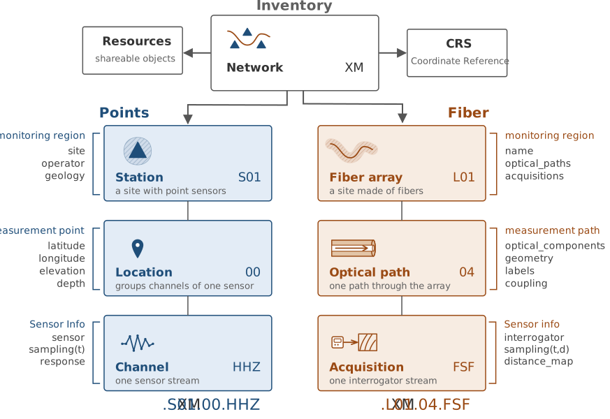
This is a conceptual comparison with StationXML, not a literal containment diagram. In DASCore, acquisitions and optical paths are sibling collections on a fiber array. There is no Location model: a Channel carries a location_code, and a station holds its channels directly.

An Inventory contains Network objects. A network may hold conventional stations and FiberArray objects. Each fiber array holds:

• Acquisition objects, which describe an interrogator stream and map instrument distance onto an optical path.
• OpticalPath objects, which describe what the light travelled through.

Shared objects such as interrogators, cables, enclosures, and measurements live under Inventory.resources. Other objects refer to them by resource_id, avoiding duplicate metadata; model constructors also accept the object itself.

In notebook displays, a long model description appears as description: …. Open a leaf model to read it, or open the description within a model that has children. Short descriptions remain in the summary line.

Optical-path track concepts.

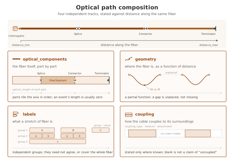
An optical path has four independent tracks along optical distance:

• optical_components: fiber segments, splices, connectors, amplifiers, and terminators. These tile the complete path and define its extent.
• geometry: measured quantities along the fiber, including coordinates named by the inventory’s coordinate reference system.
• coupling: how each interval of cable meets its surroundings.
• labels: interval names such as borehole, drift, or zone.

Geometry, coupling, and labels may cover only part of the path. Missing coverage means “not stated,” not that the fiber or channel is absent.

Acquisitions and optical paths may have time-bounded epochs. Resolving a patch therefore uses both its acquisition key and time: hardware or geometry can change without changing the durable fiber-array identity.

Authoring an inventory

Inventories can be written as one YAML or JSON document, but a directory is easier to maintain: models use YAML or JSON, while long tracks use CSV.

inventory/
├── inventory.yaml
├── resources/
│   └── interrogator-1.yaml
├── acquisitions/
│   └── DAS.R2D1..RAW.yaml
└── fiber_arrays/
    └── DAS.R2D1/
        ├── attrs.yaml
        └── path/
            ├── attrs.yaml
            ├── optical_components.csv
            ├── geometry.csv
            ├── coupling.csv
            └── labels.csv

Each object file declares its object_type. An acquisition filename gives its full identity, and its distance_map connects the interrogator’s axis to optical distance:

object_type: Acquisition
data_category: DAS
data_type: velocity
gauge_length: 10.0
interrogator: interrogator-1
distance_map:
  instrument_distance: [0.0, 299.0]
  distance: [100.0, 399.0]

Track files are ordinary tables. For example:

object_type,distance_min,distance_max,name
FiberSegment,0,100,lead-in
Splice,100,,wellhead splice
FiberSegment,100,500,trench cable

A point component leaves distance_max blank; a fiber segment states both bounds. Rows are ordered by distance when loaded, regardless of file order.

The main authoring rules are:

• File and directory names state identity. If the file repeats an identity field, the values must agree.
• path is the reserved optical-path directory. attrs and inventory are reserved file stems.
• Files outside reserved object slots are ignored unless they declare a recognized inventory object; files inside reserved slots must follow the conventions. Field notes and photographs may live elsewhere in the inventory tree.
• CSV columns beginning with _ are also ignored. Use description for notes that should survive serialization.
• Quantities that interpolate belong in geometry.csv; interval values belong in labels.csv. Units may appear in geometry headers, for example chainage (m).

A dated entity uses an @time suffix, such as path@2025-01-01/, to begin a new epoch. The directory loader validates identities, object types, references, track coverage, and epoch ranges when dc.inventory reads it.

Position is ordinary geometry whose column names match the coordinate reference system, or the canonical aliases x, y, and z. Positional axes must be stated together and use the CRS units; a geometry segment may omit all of them and record another quantity such as chainage instead. Fiber gathered at one place, such as a spool, is a segment of two rows with the same position at the spool’s start and end distances. Segments that place the axes may not overlap in optical distance.

The tunnel inventory recipe builds a complete directory, including resources, geometry, repairs, and multiple optical paths.

Track semantics

Tracks use three shapes:

shape	tracks	coverage	overlap	value outside coverage
tiling	optical_components	complete	none	—
function	geometry columns, coupling, labels with values	partial	none	"" or NaN
membership	labels without values	partial	allowed	False

Every label names its group, the coordinate it becomes. A label with an empty value states membership; a label with a value defines an interval coordinate. Literal true and false values are refused because an empty value already spells membership. One label group must consistently contain text, numbers, or membership. Numeric groups use NaN outside coverage and therefore project as floating-point coordinates.

Intervals are half-open, [start, end), so adjacent rows can tile without overlap. Projection still includes the final channel at the end of a covered run.

Geometry columns, label groups, and typed tracks become coordinates. Label group names cannot use structural names, track names, or recognized coordinate labels; see RESERVED_GROUP_NAMES in dascore.core.inventory. Geometry columns may use coordinate labels—that is how a segment states an axis—but cannot share a name with a label group.

Inspecting and visualizing

The examples below use an inventory and patch designed to resolve together:

import tempfile
from pathlib import Path

import dascore as dc
from dascore.examples import inventory_patch_pair
from dascore.exceptions import PatchError

patch, inventory = inventory_patch_pair()

Inventory.get_names separates scalar attributes from per-channel coordinates:

names = inventory.get_names()
assert "gauge_length" in names.attrs
assert {"zone", "noisy", "coupling"} <= set(names.coords)

The result lists what the inventory can contribute, not what every channel will receive. A partially covered path may list a coordinate whose value is blank for some channels.

Inventory.viz.path aligns acquisitions, components, coupling, labels, and geometry along optical distance:

inventory.viz.path(show=True);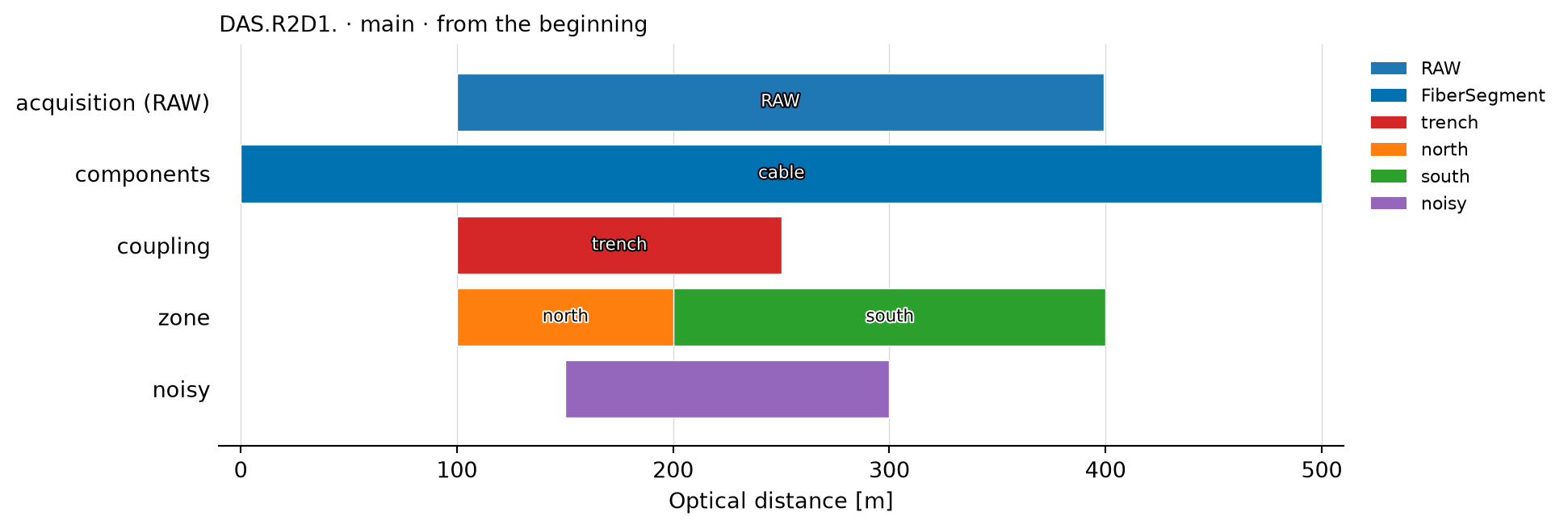

Use tracks= to select lanes and columns= to select geometry columns. Inventory.viz.map plots geometry in space, while Inventory.viz.timeline plots acquisition and path epochs through time.

Using an inventory with a spool

Spool.attach_inventory stores an inventory reference without changing patches or loading data. enrich can also take an inventory, which it attaches; without one it uses the attached inventory, as conform_to_inventory always does.

spool = dc.spool(patch).attach_inventory(inventory)
assert "gauge_length" not in dict(spool[0].attrs)

Once attached, inventory coordinates can drive selection and expansion:

northern = spool.select(zone="north")
zones = spool.expand_by("zone")
assert set(zones.get_contents()["zone"]) == {"north", "south"}

Selection trims channels; a patch with no matching channels drops out.

Selection and expansion also drop a patch that no single inventory context describes: one straddling an acquisition or optical-path change, reaching outside every optical-path epoch, or not described at all; unselect keeps it. A straddling patch’s parts could answer differently, and selection judges whole patches rather than splitting them, so each call warns once with the number of such patches. Run conform_to_inventory first: it splits patches at optical-path changes so each described part can be selected, and by default raises on the rest; pass on_unresolved="ignore" to drop them. It refuses a patch spanning an acquisition change; select the time on each side of the change instead. A patch that resolves but does not match drops out silently. The same holds for an inventory-backed attribute such as gauge_length, unless the patch states it in its own header.

Attaching a replacement inventory clears enrichment configured from the old one, preventing stale instructions from being applied to new metadata.

Enriching patches

Spool.enrich copies resolved metadata as patches are loaded. Acquisition and interrogator facts become attributes; optical-path facts become per-channel coordinates.

enriched = spool.enrich()[0]
assert enriched.attrs.gauge_length == 10.0
assert "zone" in enriched.coords.coord_map
assert set(enriched.get_array("coupling")) == {"trench", ""}

The acquisition’s distance_map performs the projection. Compatible distance units are converted; incompatible axes raise. With two or more control points, channels outside the map’s range are not placed; with one, the map extends in both directions, by spatial_interval per channel on the channel axis (which therefore needs spatial_interval) and one meter per meter on the instrument_distance axis. Channels that are not placed, or are placed beyond the ends of the optical path, get no coordinates from the path’s tracks (NaN, or empty for text). This is normal for an interrogator that records past the end of the fiber, so it is not reported. An unresolved patch is returned unchanged with a warning, so enrichment never silently removes data.

By default, scalar acquisition fields and interrogator.* fields become attributes, while geometry, coupling, and labels become coordinates. Position coordinates take the names the inventory’s coordinate reference system declares, such as easting, northing, and elevation; an inventory left with the default CRS gets x, y, and z, and either spelling can be requested by name. data_type and data_units are excluded because processing may have changed the data; sample_rate and spatial_interval are excluded because the patch coordinates already state them. They can still be requested explicitly.

Unset attributes are always filled. If a stated patch attribute conflicts with the inventory, conflict chooses the result: raise (default) reports the contradiction, since it usually means the patch resolved to the wrong acquisition; keep_first keeps the patch value, keep_last uses the inventory, and drop removes both.

stale = patch.update_attrs(gauge_length=99.0)
try:
    stale.enrich(inventory)
except PatchError as err:
    print(err)
assert stale.enrich(inventory, conflict="keep_first").attrs.gauge_length == 99.0
assert stale.enrich(inventory, conflict="keep_last").attrs.gauge_length == 10.0

The patch's 'gauge_length' is 99.0 but the inventory says 10.0. A disagreement here usually means the acquisition_key resolved to the wrong place.

Patch.enrich performs the same operation directly on one patch, but an unresolved patch raises instead of using the spool’s on_unresolved policy.

Conforming a spool

Spool.conform_to_inventory eagerly resolves every row, rejects or drops unresolved patches, and subdivides patches at optical-path changes. Unlike attachment and enrichment, it can change spool length.

stranger = dc.get_example_patch("random_das", acquisition_key="XX.NOPE..RAW")
mixed = dc.spool([patch, stranger]).attach_inventory(inventory)

conformed = mixed.conform_to_inventory(on_unresolved="ignore")
assert len(conformed) == 1
assert conformed[0].attrs.acquisition_key == "DAS.R2D1..RAW"

Subdivision preserves every sample exactly once. A patch with any sample outside every acquisition epoch, or outside every optical-path epoch at its location, is unresolved as a whole rather than cut. An acquisition whose location never has an optical path is exempt, since it is pathless by design. Use on_unresolved="warn" or "ignore" when an inventory intentionally covers only part of an archive.

Conforming raises when one patch straddles an acquisition change, since a patch cannot carry two acquisition configurations. This is why attachment remains inert: conforming can remove, split, or reject data and must be requested explicitly.

Inventory files beside data

A data directory may carry its inventory as .inventory/, .inventory.yaml, .inventory.yml, or .inventory.json. A spool opened on that directory attaches it automatically:

data_path = Path(tempfile.mkdtemp()) / "archive"
data_path.mkdir()
patch.io.write(data_path / "patch.h5", "DASDAE")
inventory.io.to_yaml(data_path / ".inventory.yaml")

carrying = dc.spool(data_path).update()
assert carrying.enrich()[0].attrs.gauge_length == 10.0

Discovery happens when the spool opens, but parsing waits until an inventory-backed operation. Ordinary len, sorting, chunking, patch loading, and selection using only indexed names do not parse it; selection on an inventory coordinate does. The inventory is then cached. After editing it, call attach_inventory() with no argument to reread the directory’s copy.

Two .inventory spellings in one directory are refused as ambiguous. The visible name inventory.yaml is not a companion file: in the authoring format it is the inventory envelope.

Serializing

Inventory.io.to_yaml produces the single-file interchange form. dc.inventory reads directory, YAML, JSON, model, or serialized text inputs.

text = inventory.io.to_yaml()
assert dc.inventory(text) == inventory

json_path = data_path / "inventory.json"
json_path.write_text(inventory.model_dump_json())
assert dc.inventory(json_path) == inventory

Invalid documents consistently raise InvalidInventoryError.