import numpy as np

import dascore as dc

patch = dc.get_example_patch()Patch Processing
Keywords
filtering, processing, signal processing
Patch-processing methods return new patches and are listed in the dascore.proc API.
Shape and missing values
transpose changes dimension order, squeeze removes length-one dimensions, and dropna removes labels containing null values.
transposed = patch.transpose("time", "distance")

flat = patch.select(distance=0, samples=True)
squeezed = flat.squeeze()

data = np.array(patch.data)
data[:, 0] = np.nan
without_nan = patch.new(data=data).dropna("time")
transpose() with no arguments rotates dimension order. squeeze() can name dimensions to remove and rejects any named dimension whose length is not one. dropna keeps coordinate and data indexing synchronized.
Decimate
Patch.decimate downsamples a dimension and applies an anti-aliasing filter by default.
waves = dc.examples.get_example_patch(
    "sin_wav",
    sample_rate=1000,
    frequency=[200, 10],
    channel_count=2,
)

iir = waves.decimate(time=10, filter_type="iir")
fir = waves.decimate(time=10, filter_type="fir")
aliased = waves.decimate(time=10, filter_type=None)
Use filter_type=None only when aliasing is intentional or filtering has already been performed.
iir.viz.wiggle(show=True);
aliased.viz.wiggle(show=True);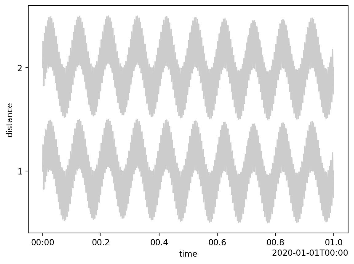
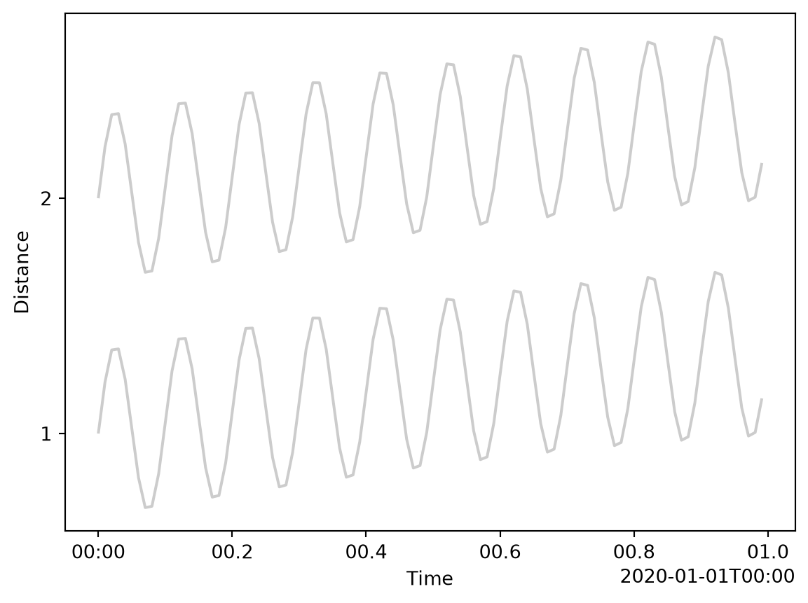
Here the filtered result removes the 200 Hz component before reducing the 1,000 Hz sample rate. The unfiltered result folds that energy into a lower apparent frequency.
Taper
Patch.taper applies a cosine taper to a fraction of a dimension. A tuple controls the two ends; None leaves one end unchanged.
ones = patch.new(data=np.ones_like(patch.data))
both_ends = ones.taper(time=0.1)
different_ends = ones.taper(distance=(0.1, 0.3))
end_only = ones.taper(distance=(None, 0.1))different_ends.viz.waterfall(show=True);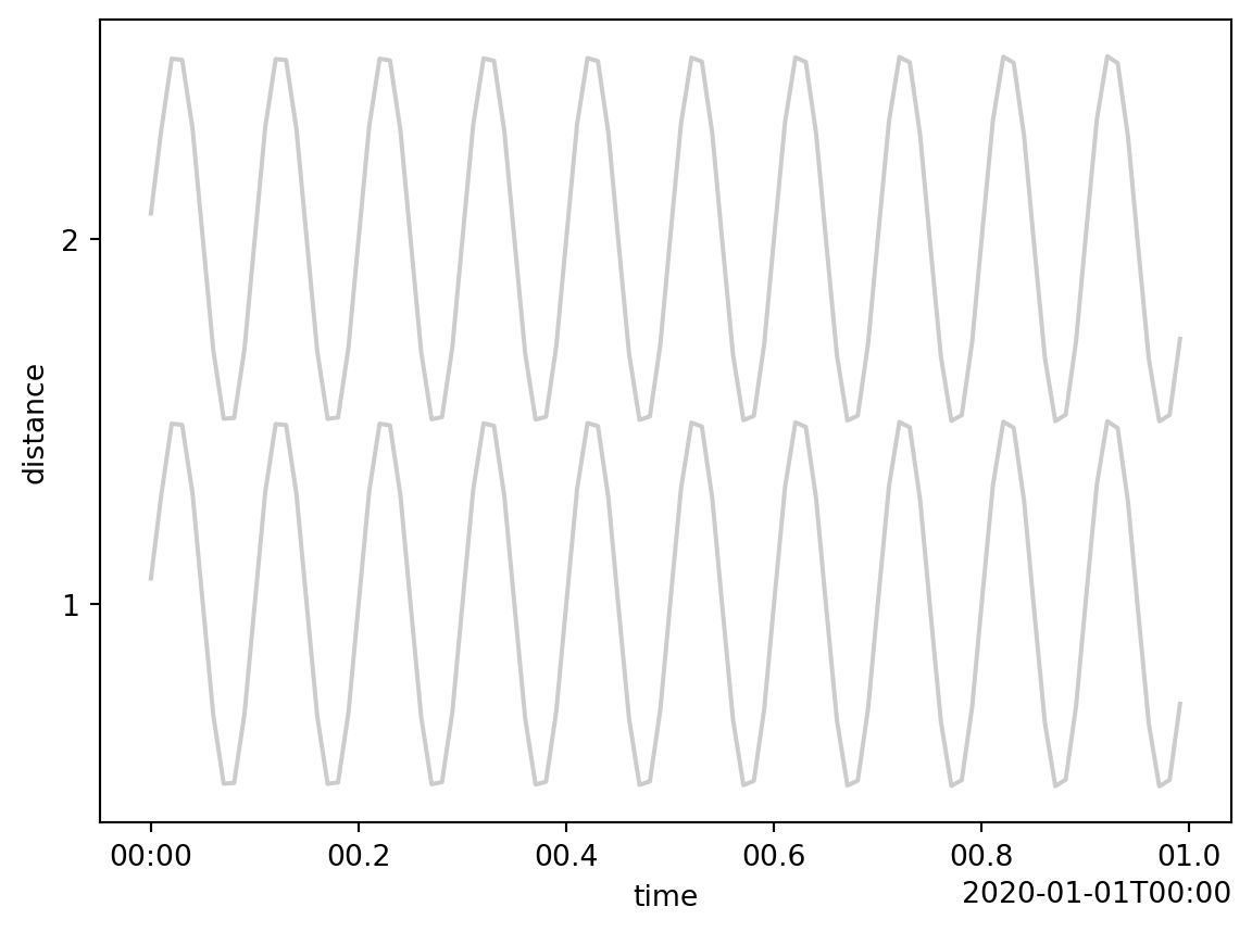
A scalar applies the same fraction at both ends. Tuple values let asymmetric records taper more strongly at one boundary, and may also be expressed with compatible units where supported.
See the edge-effects recipe for tapering before filters.
Rolling windows
Patch.rolling provides moving-window reductions. Incomplete windows produce NaNs, which can be removed with dropna.
event = dc.get_example_patch("example_event_1")
smoothed = event.rolling(time=50, samples=True).mean().dropna("time")smoothed.viz.waterfall(show=True);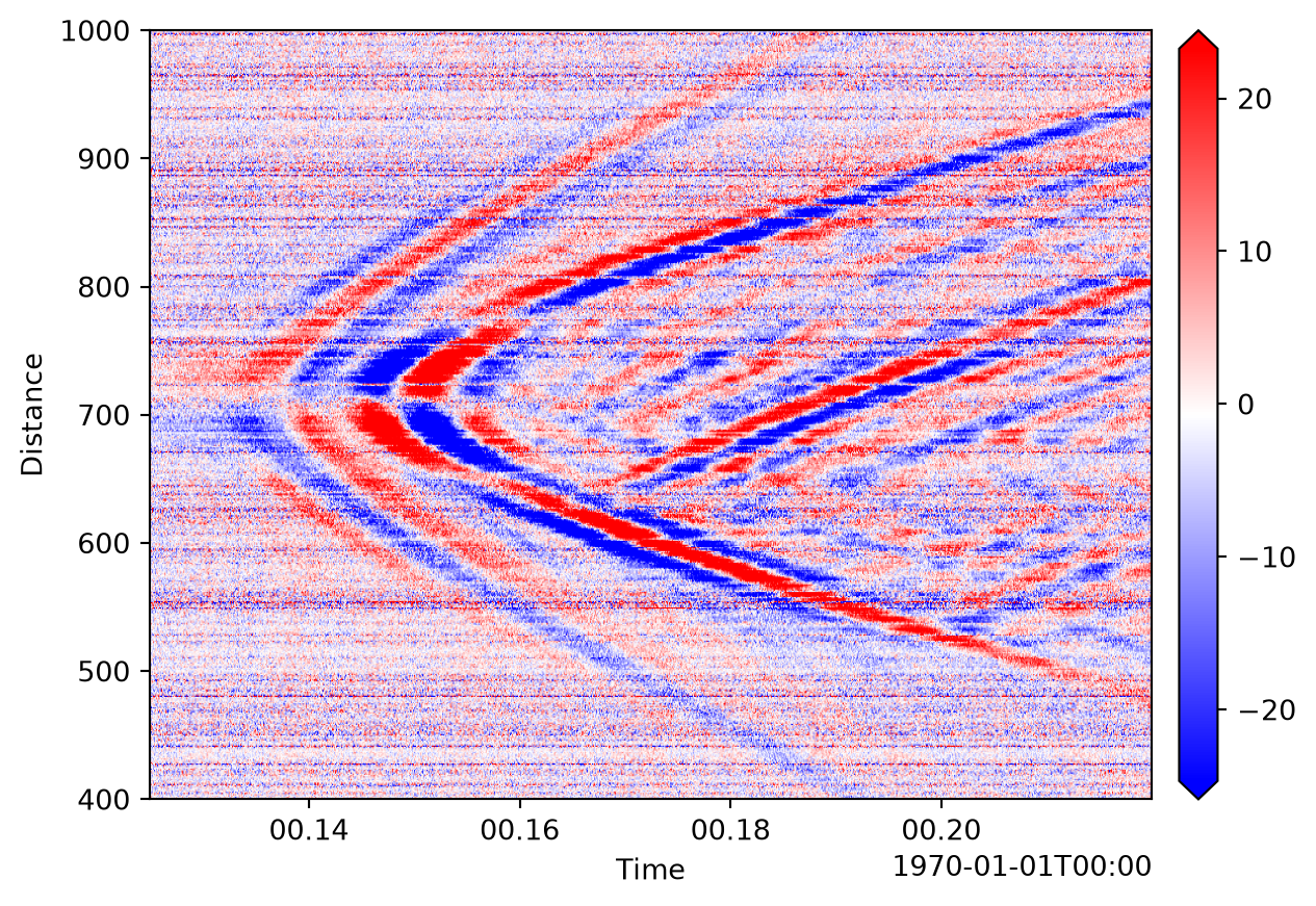
Rolling objects provide reductions such as mean, median, min, max, std, and sum. Specify a coordinate-unit window or set samples=True for an exact sample count.
Gain
Automatic gain control
Passing window to Patch.normalize divides every sample by a centered local norm. This raises weak arrivals but removes amplitude comparability across the record.
gained = event.normalize("time", norm="l2", window=0.1)gained.viz.waterfall(scale=0.5, show=True);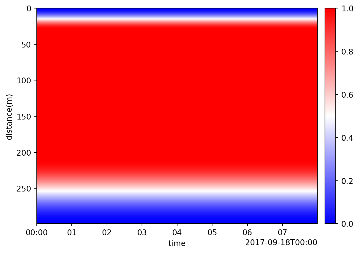
norm may be l2 (RMS), l1 (mean absolute value), or max. Window length uses coordinate units unless samples=True. Reflected edge values keep the output shape and avoid the incomplete-window NaNs produced by rolling.
Without window, normalize uses one norm for the complete trace. With a window, every sample receives its own local scale. This distinction matters when amplitudes themselves carry scientific meaning.
Power gain
Patch.pow_coord multiplies data by a coordinate raised to a power. Because the curve depends only on position, relative amplitudes remain comparable between traces.
spread_corrected = event.pow_coord(time=2)
both_dimensions = event.pow_coord(time=2, distance=1)
The coordinate count begins at one rather than zero, so the first sample retains its amplitude. Time powers of one or two are common geometric-spreading corrections; other dimensions can be corrected in the same call.
Whiten
The Patch.whiten function performs spectral whitening by balancing the amplitude spectra of the patch while leaving the phase (largely) unchanged. Spectral whitening is often a pre-processing step in ambient noise correlation workflows.
To demonstrate, we create some plotting code and an example patch.
import matplotlib.pyplot as plt
import numpy as np

import dascore as dc
from dascore.utils.time import to_float


rng = np.random.default_rng()


def plot_time_and_frequency(patch, channel=0):
    """ Make plots of time and frequency of patch with single channel."""
    sq_patch = patch.select(distance=channel, samples=True).squeeze()
    time_array = to_float(patch.get_array("time"))
    time = time_array - np.min(time_array)

    fig, (td_ax, fd_ax, phase_ax) = plt.subplots(1, 3, figsize=(9, 2.5))

    # Plot in time domain
    td_ax.plot(time, sq_patch.data, color="tab:blue")
    td_ax.set_title("Time Domain")
    td_ax.set_xlabel("time (s)")

    # Plot freq amplitdue
    ft_patch = sq_patch.dft("time", real=True)
    freq = ft_patch.get_array("ft_time")
    fd_ax.plot(freq, ft_patch.abs().data, color="tab:red")
    fd_ax.set_xlabel("Frequency (Hz)")
    fd_ax.set_title("Amplitude Spectra")

    # plot freq phase
    phase_ax.plot(freq, np.angle(ft_patch.data), color="tab:cyan")
    phase_ax.set_xlabel("Frequency (Hz)")
    phase_ax.set_title("Phase Angle")

    # fd_ax.set_xlim(0, 1000)
    return fig


def make_noisy_sine_patch():
    """Make a noisy sine wave patch."""
    patch = dc.get_example_patch(
        "sin_wav",
        frequency=[1, 10, 20, 54, 66],
        amplitude=[1, 2, 3, 4, 9],
        duration=1,
        sample_rate=200,
    )
    rand_noise = (rng.random(patch.data.shape) - 0.5) * 10
    patch = patch.new(data = patch.data + rand_noise)
    return patch
patch = make_noisy_sine_patch()
plot_time_and_frequency(patch);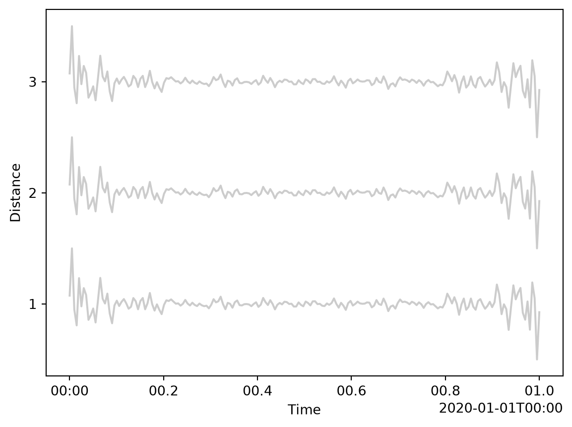
The default whitening makes all spectral amplitudes equal.
white_patch = patch.whiten()
plot_time_and_frequency(white_patch);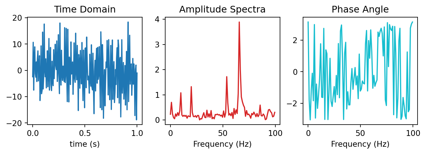
The whitening can be restricted to certain frequency bands by specifying the dimension and a frequency range.
white_patch = patch.whiten(time=(20, 80))
plot_time_and_frequency(white_patch);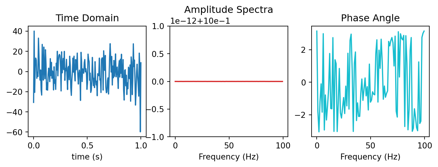
Four values can be used to control the start/end of the taper.
white_patch = patch.whiten(time=(20, 40, 60, 80))
plot_time_and_frequency(white_patch);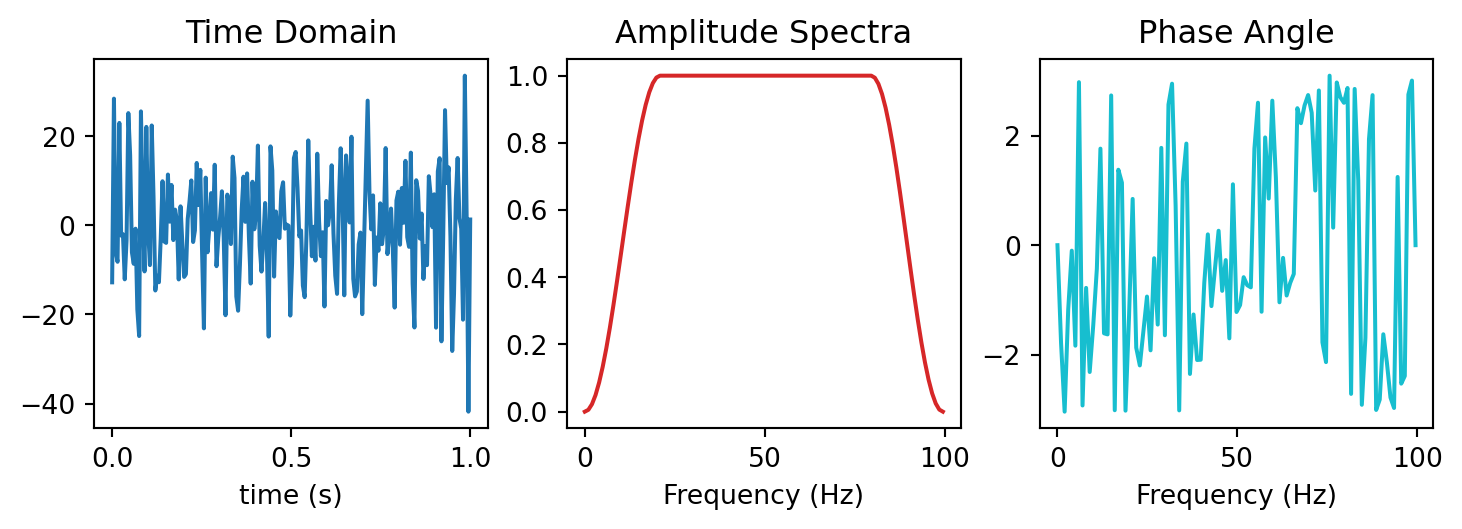
Whiten also supports using a smoothed amplitude for normalization which causes less drastic changes to the amplitude spectrum.
white_patch = patch.whiten(smooth_size=1)
_ = plot_time_and_frequency(white_patch)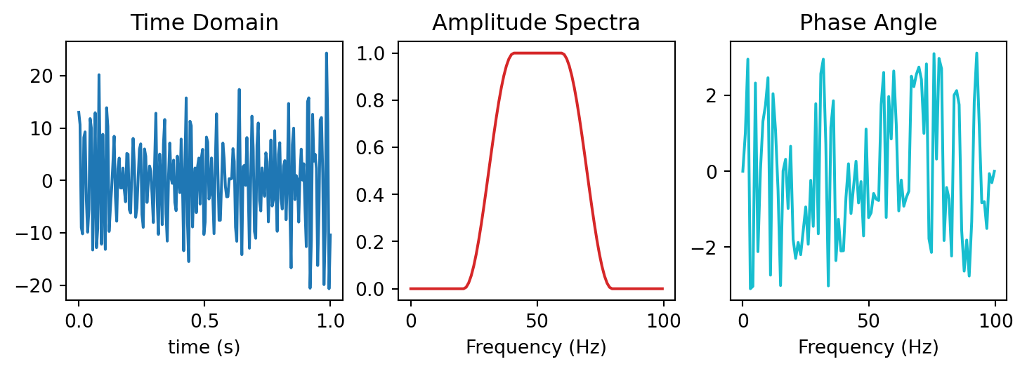
white_patch = patch.whiten(smooth_size=2, time=(10, 20, 80, 90))
_ = plot_time_and_frequency(white_patch)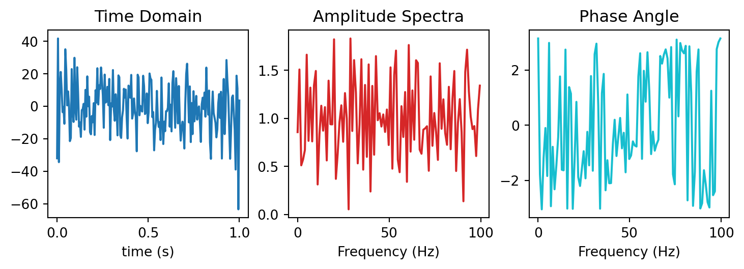
Whiten also accepts patches in the frequency domain, in which case frequency patches are returned. This might be useful if whiten is only a part of a frequency domain workflow.
fft_patch = patch.dft("time", real=True)
dft_white = fft_patch.whiten(smooth_size=1, time=(20, 40, 60, 80))
td_patch = dft_white.idft()
plot_time_and_frequency(td_patch);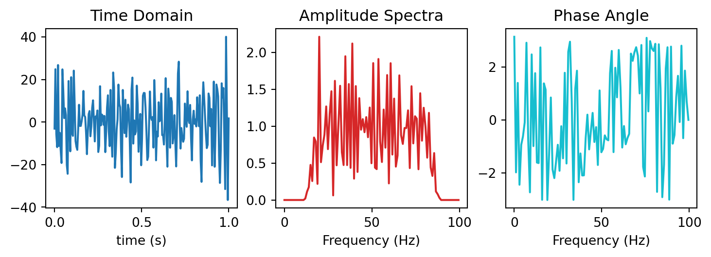
The water_level parameter can be useful for stabilizing frequencies that may have near-zero values.