import dascore as dc

patch = dc.get_example_patch("example_event_2")
patch.viz.waterfall(show=True);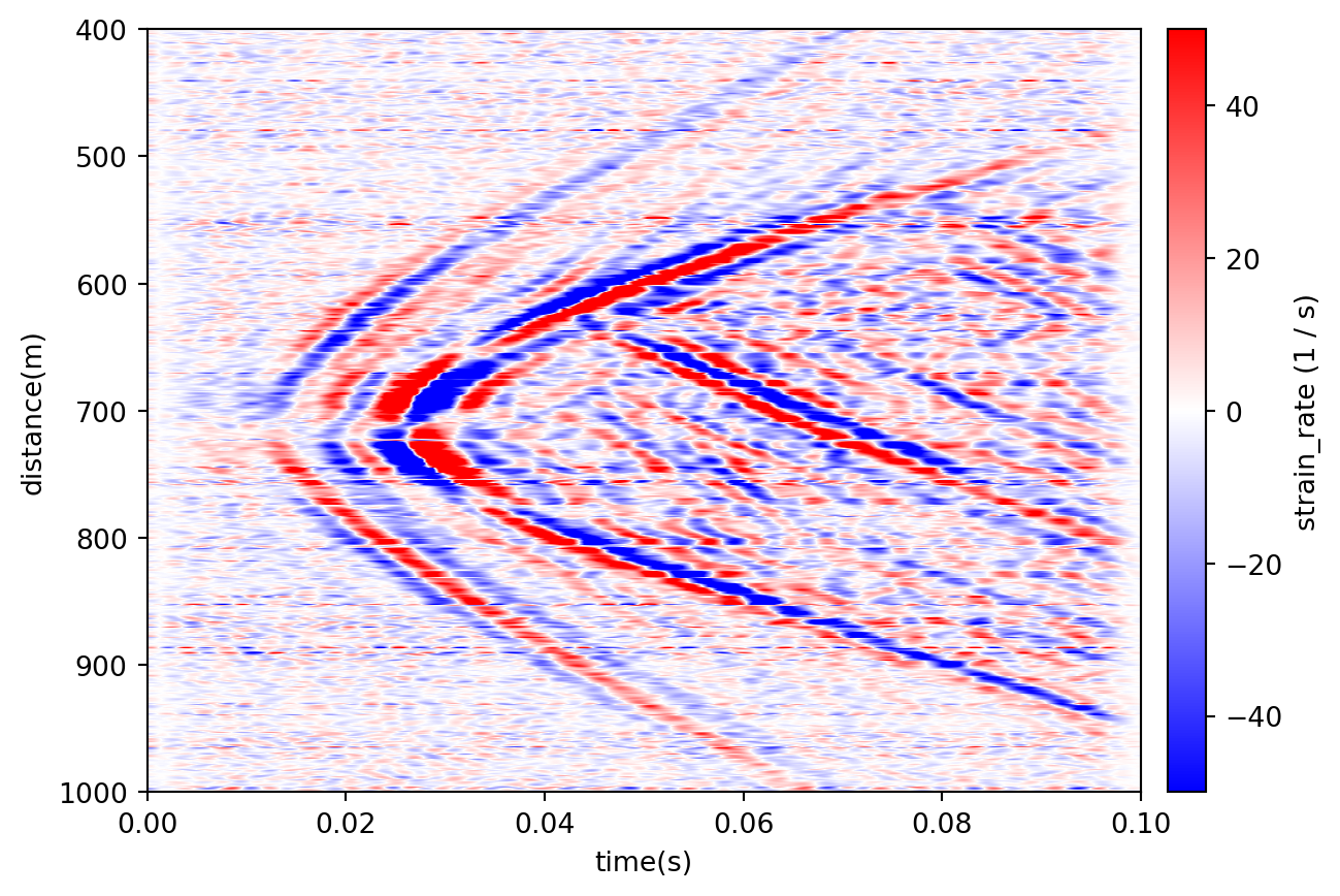
DASCore plots are available from the object they describe: Patch.viz, Spool.viz, and Inventory.viz.
Patch.viz.waterfall plots patch data as an image. Its default color limits clip to 1.5×IQR beyond the quartiles, so outliers saturate; pass scale=(0, 1) to show the full data range.
import dascore as dc
patch = dc.get_example_patch("example_event_2")
patch.viz.waterfall(show=True);
scale_type="relative" interprets scale as a fraction of the dynamic range around the mean. scale_type="absolute" accepts explicit limits.
import matplotlib.pyplot as plt

fig, (ax1, ax2) = plt.subplots(1, 2, figsize=(12, 4))
patch.viz.waterfall(scale=0.2, scale_type="relative", ax=ax1)
patch.viz.waterfall(scale=(-50, 50), scale_type="absolute", ax=ax2)
ax1.set_title("Relative")
ax2.set_title("Absolute")
plt.tight_layout()
plt.show()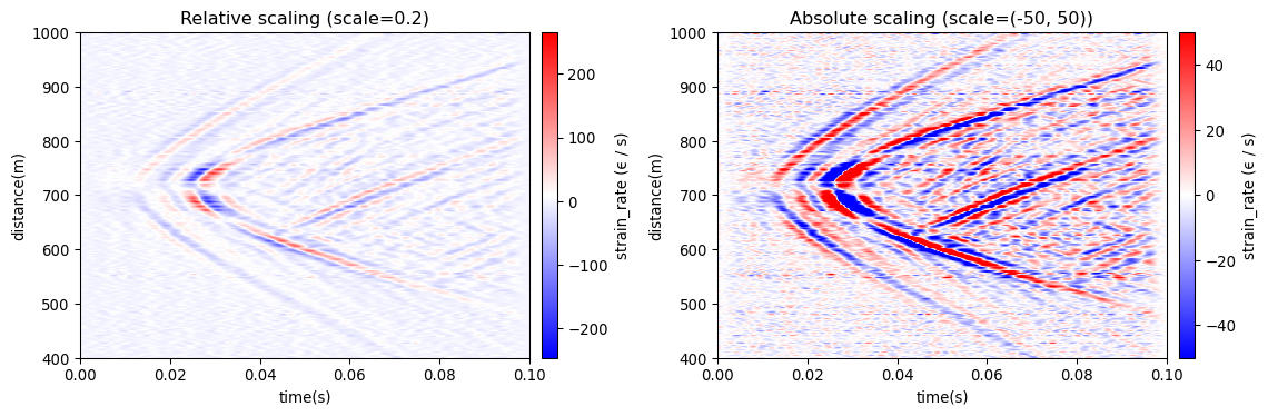
Pass an existing Matplotlib axis to compose the plot with other panels. The returned axis can be customized with the normal Matplotlib API.
Most DAS patches have more samples than the figure has pixels, so Matplotlib has to downsample them, and interpolation_stage decides how. "data" averages the data first and then colors the result; "rgba" colors every sample first and then averages the colors. The default, "auto", uses "rgba" whenever it downsamples. This applies to evenly sampled patches, which are drawn with imshow; irregular coordinates use pcolormesh, which ignores interpolation_stage.
Neither is right for every patch. In the top row below, "data" keeps the strong contrast of the arrivals, while "rgba" blends neighbouring reds and blues into paler colors. In the bottom row, the same patch carries an oscillation far faster than one pixel: "data" averages it away, hiding that it exists, while "rgba" shows it as a grey wash.
import numpy as np

base = dc.get_example_patch("example_event_2")
big = base.resample(time=base.get_coord("time").step / 10)
time = big.get_array("time")
carrier = 40 * np.sin(2 * np.pi * 20_000 * (time - time[0]))
noisy = big.new(data=big.data + carrier[None, :])

fig, axes = plt.subplots(2, 2, figsize=(12, 8))
for row, plot_patch in zip(axes, [big, noisy]):
    for ax, stage in zip(row, ["data", "rgba"]):
        plot_patch.viz.waterfall(ax=ax, interpolation_stage=stage)
        ax.set_title(f'interpolation_stage="{stage}"')
plt.tight_layout()
plt.show()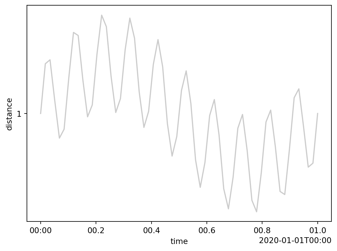
Try "data" when coherent arrivals look washed out, and "rgba" when the image looks suspiciously clean. Low-pass filtering and then decimating the patch to about the figure’s pixel count avoids the question, since nothing is left to downsample.
After Patch.enrich adds inventory labels as coordinates, label_coord marks their ranges along the plot edges. Boolean coordinates mark membership under their coordinate name.
from dascore.examples import inventory_patch_pair

zoned, inventory = inventory_patch_pair()
zoned.enrich(inventory).viz.waterfall(label_coord="zone", show=True);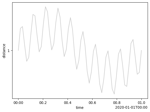
Labels are drawn on both spines of their associated dimension, with faint lines across the image at value changes. Missing labels leave the spine bare. Coordinates associated with time use the top and bottom spines; distance coordinates use the left and right.
zoned.enrich(inventory).viz.waterfall(label_coord="noisy", show=True);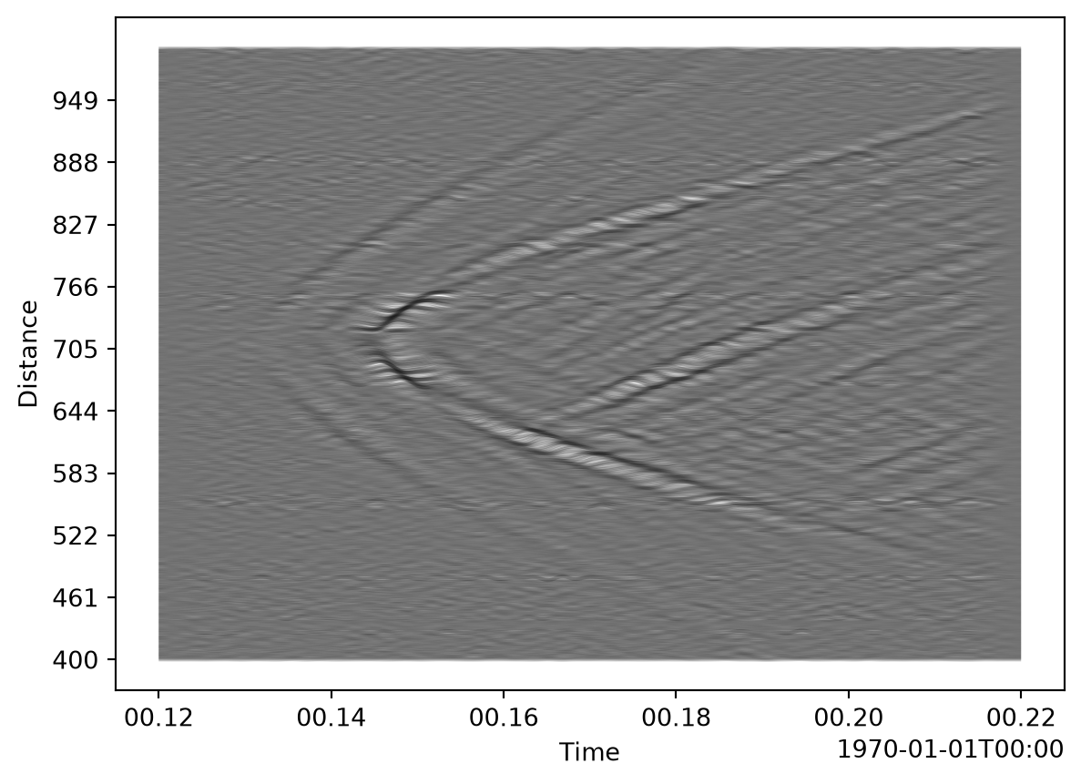
Patch.viz.wiggle draws offset traces. Time-like stacking axes are inverted; other axes retain their normal direction.
The default stacks traces along distance, leaving positive amplitudes upward. If traces are stacked along time, the time axis is inverted and positive amplitudes point right in the conventional display.
event = (
    dc.get_example_patch("example_event_1")
    .taper(time=0.05)
    .pass_filter(time=(..., 300))
)
event.viz.wiggle(scale=0.5, show=True);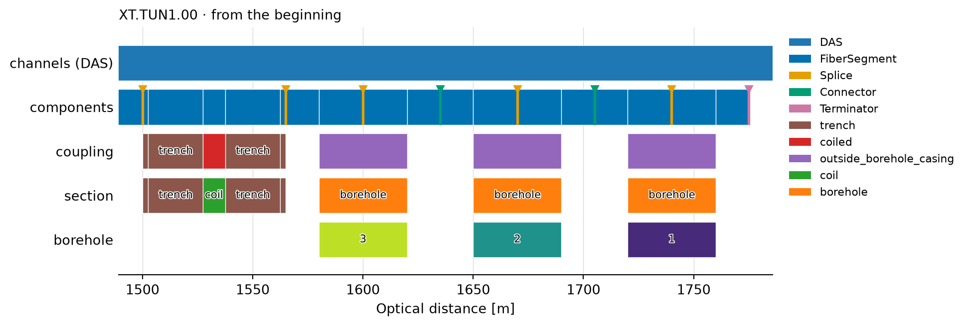
Inventory plots show the observing system without loading patch data. These examples use the deployment from the tunnel inventory recipe.
inventory = dc.get_example_inventory("tunnel")Inventory.viz.path draws each track against optical distance. Use distance= to focus on part of the fiber.
inventory.viz.path(time="2024-07-01", distance=(1495, 1780), show=True);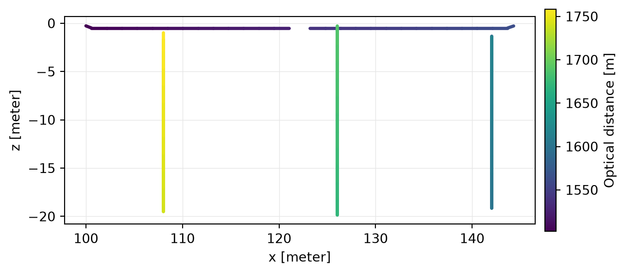
Tracks are drawn in optical order. Point features such as splices appear as ticks, while intervals such as boreholes occupy their measured spans.
Inventory.viz.map draws two physical coordinates. color= accepts optical distance, coupling, geometry columns, or label groups. Unsurveyed fiber is left as a gap.
inventory.viz.map(x="x", y="z", color="section", time="2024-07-01", show=True);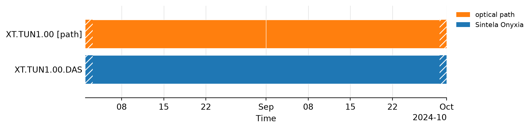
The default color is optical distance, which links a distance read from a waterfall to its physical location. Choose x and y for the useful view; a vertical borehole collapses to a point in plan view.
Inventory.viz.timeline shows when acquisitions and optical paths are valid. Hatched ends indicate unbounded epochs.
inventory.viz.timeline(show=True);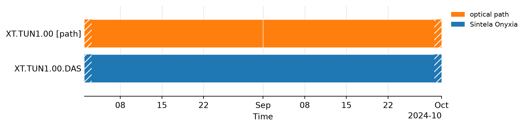
Open-ended validity intervals continue beyond the corresponding side of the axis. Use the timeline before selecting a time= for the path or map when an inventory contains several configurations.
Spool plots use index metadata, so they do not load patch arrays.
spool = dc.get_example_spool("sparse_dss")Spool.viz.coverage gives each compatible patch group a lane showing its runs, gaps, and coverage percentage. It uses the same grouping and gaps as get_coverage and get_gaps.
spool.viz.coverage(show=True);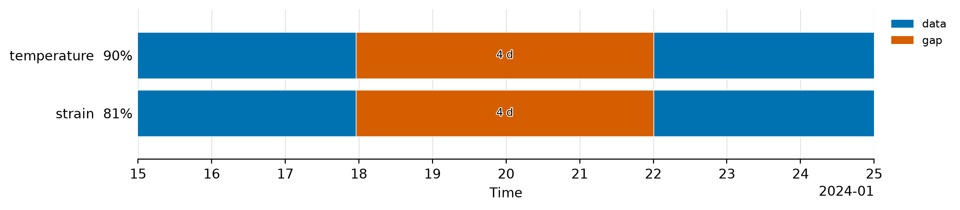
Lane names contain the metadata that separates compatible groups and append that group’s coverage. A spool representation uses the same kind attributes for tracks, but coverage lanes may split a track further by sampling rate or coordinate structure.
Time is the default dimension; pass another one as in spool.viz.coverage("distance"). Select a smaller spool before plotting when coverage percentages should describe a smaller window; change only the axes to zoom without changing the statistics.
spool.select(time=("2024-01-15", "2024-01-25")).viz.coverage(show=True);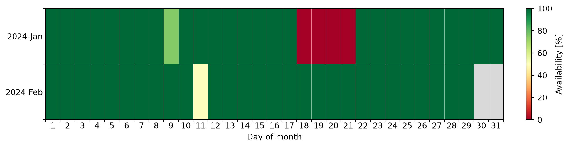
Setting axis limits instead keeps the full-spool percentages and only changes the viewport. A line continuing beyond an axis edge then correctly indicates data outside the visible window.
import numpy as np

ax = spool.viz.coverage()
ax.set_xlim(np.datetime64("2024-01-15"), np.datetime64("2024-01-25"));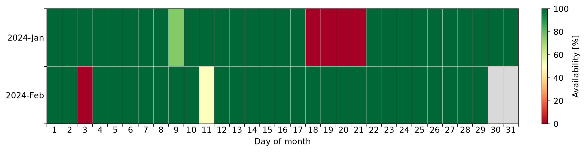
Spool.viz.calendar summarizes long time ranges by day. Each cell is the union of all selected patch groups and cannot exceed 100%; grey cells are invalid calendar dates.
spool.viz.calendar(show=True);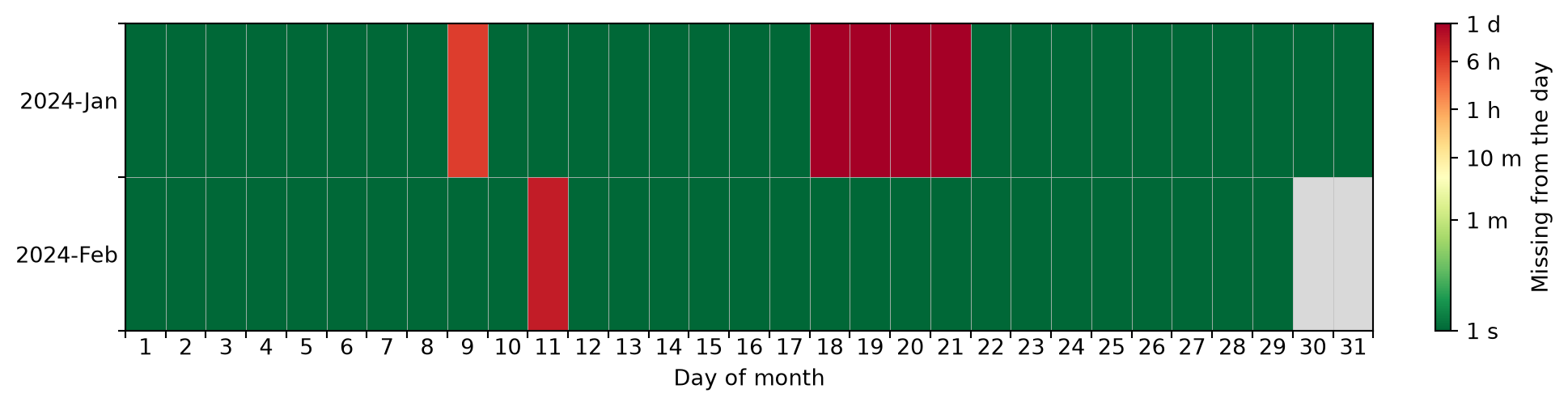
Because each day is a union, simultaneous acquisitions do not count twice. Empty valid dates represent no coverage; grey cells represent dates which do not exist, such as February 30.
Select an acquisition before plotting it alone. Use method="gap" to emphasize short gaps or method="count" to show overlapping patch counts.
spool.select(tag="temperature").viz.calendar(show=True);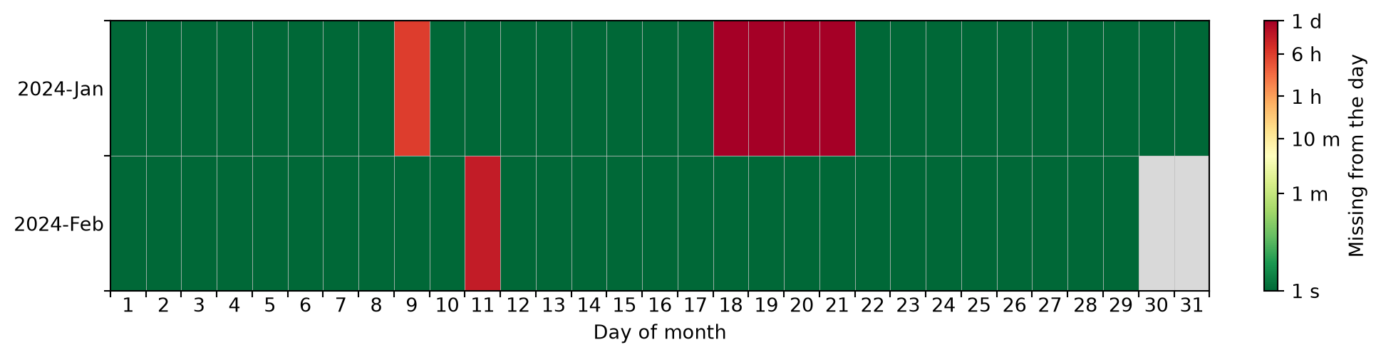
spool.viz.calendar(method="gap", show=True);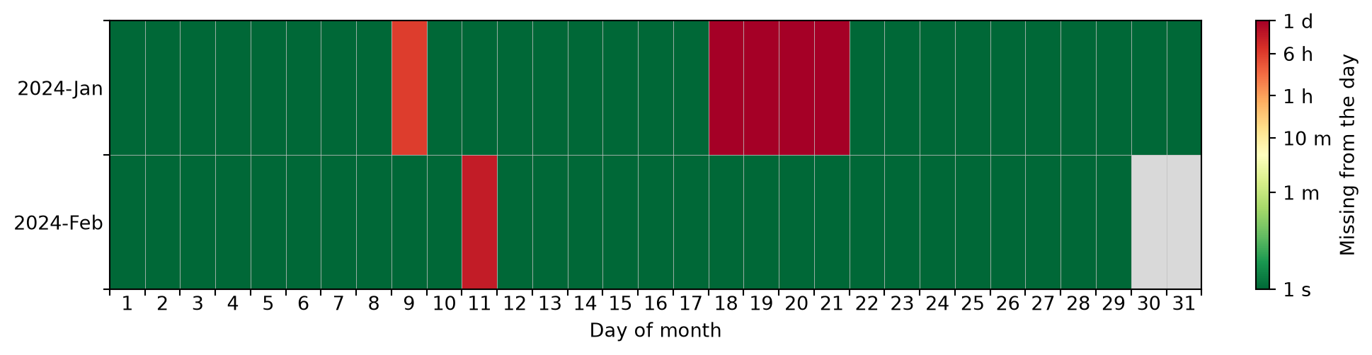
The group argument controls which boundaries count as gaps; it does not select an acquisition. Filter the spool first when the calendar should describe only part of the archive.