import dascore as dc
patch = dc.get_example_patch()

# Create a spectrogram plot
ax = patch.viz.spectrogram(show=False)

# Half second windows, zero padded to 512 point FFTs, log colours.
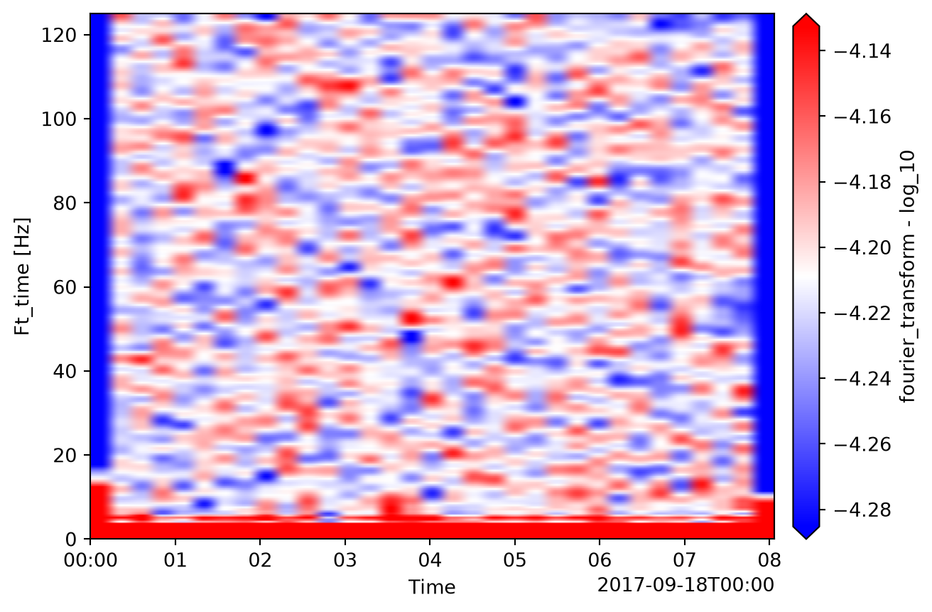
ax = patch.viz.spectrogram(time=0.5, nfft=512, log=True)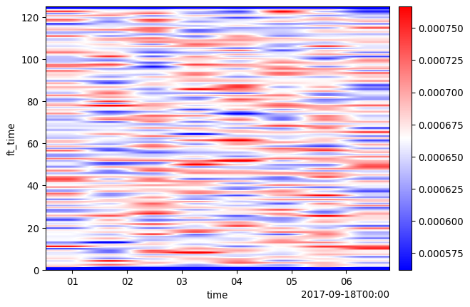
spectrogram(
patch: Patch ,
ax: matplotlib.axes._axes.Axes | None[Axes, None] = None,
dim = time,
aggr_domain = frequency,
cmap = bwr,
scale: float | collections.abc.Sequence[float, collections.abc.Sequence[float], None] = None,
scale_type: Literal[‘relative’, ‘absolute’] = relative,
log = False,
show = False,
taper_window: Any = hann,
overlap: pint.registry.Quantity | int | None[Quantity, int, None] = 50 %,
nfft: int | pint.registry.Quantity | None[int, Quantity, None] = None,
samples: bool = False,
detrend: bool = False,
**kwargs ,
)-> ‘plt.Axes’
Plot a spectrogram of a patch.
| Parameter | Description |
|---|---|
| patch : PatchType | The Patch object. |
| ax : matplotlib.axes.Axes or None, optional | A matplotlib axis object. If None, creates a new axis. |
| dim : str, optional |
Dimension along which the spectrogram is being plotted. Default is “time”. |
| aggr_domain : str, optional |
“time” or “frequency” in which the mean value of the other dimension is calculated. No need to specify if the other dimension’s coordinate size is 1. Default is “frequency”. |
| cmap : str or matplotlib.colors.Colormap, optional |
A matplotlib colormap string or instance. Set to None to not plot the colorbar. Default is “bwr”. |
| scale : float, tuple of floats, or None, optional |
If not None, controls the saturation level of the colorbar. Values can be a single float or a length-2 tuple specifying upper and lower limits. See scale_type for more details.
|
| scale_type : {“relative”, “absolute”}, optional |
Specifies the type of scaling: - “relative”: Scale based on half the dynamic range in the patch. - “absolute”: Scale based on absolute values provided to scale.Default is “relative”. |
| log : bool, optional | If True, visualize the common logarithm of the absolute values of patch data. |
| show : bool, optional | If True, show the plot. Otherwise, just return the axis. |
| taper_window, overlap, nfft, samples, detrend | Passed to Patch.stft, and read as it reads them. |
| **kwargs |
The window, as Patch.stft takes it: the dimension and its length, such as time=0.5 (seconds) ortime=256, samples=True. With none given, a 256 sample window alongdim.
|
import dascore as dc
patch = dc.get_example_patch()
# Create a spectrogram plot
ax = patch.viz.spectrogram(show=False)
# Half second windows, zero padded to 512 point FFTs, log colours.
ax = patch.viz.spectrogram(time=0.5, nfft=512, log=True)
This is Patch.stft followed by Patch.viz.waterfall, with one other dimension averaged away, and the values drawn are |STFT|² in the scaling stft uses. Each spectrum is drawn at its window-centre label over one hop interval. The overlapping source-window bounds are omitted from this plotting view so adjacent windows cannot obscure each other. Before DASCore 0.1.22 it called scipy.signal.spectrogram directly, which differed in more than scaling: it removed the mean of each window (detrend="constant"), tapered with a ("tukey", 0.25) window, overlapped by an eighth of the window, took no windows past the ends of the data, and spelled its arguments as scipy does (nperseg, noverlap). Now the taper is hann, the overlap half, windows reach the ends as stft’s do, nothing is detrended unless detrend=True is passed through, and the window, overlap, taper and FFT length are given as stft takes them.