import dascore as dc
patch = dc.examples.example_event_2().decimate(time=10).T
spec = patch.dft("time").abs()
ax = spec.viz.specplot(cmap='turbo')
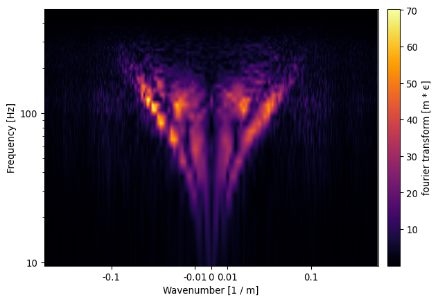
fk_patch = patch.dft(("time", "distance")).abs()
ax = fk_patch.viz.specplot(log=True, cmap='inferno')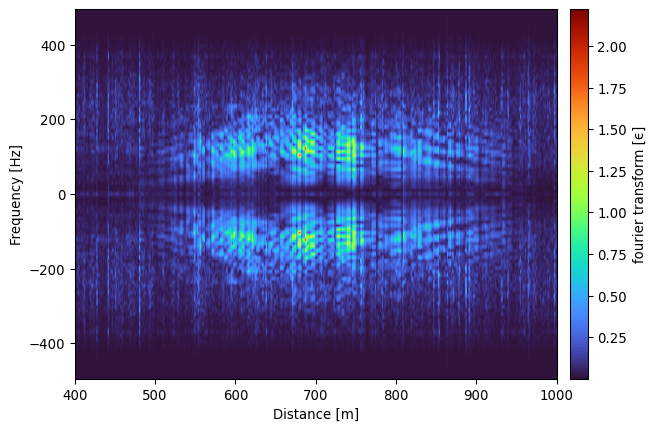
specplot(
patch: Patch ,
ax: matplotlib.axes._axes.Axes | None[Axes, None] = None,
cmap = None,
scale: float | collections.abc.Sequence[float, collections.abc.Sequence[float], None] = (0, 1),
scale_type: Literal[‘relative’, ‘absolute’] = relative,
interpolation: str | None[str, None] = bilinear,
log: bool = False,
cbar: bool = True,
show: bool = False,
**kwargs ,
)-> ‘plt.Axes’
Plot the spectrum contained in a Fourier-transformed patch.
This function wraps :meth:Patch.viz.waterfall and automatically identifies the Fourier-transformed coordinate. The corresponding axis label is replaced with a publication-friendly descriptor (e.g. Frequency or Wavenumber). Optionally, the Fourier axis can be displayed on a logarithmic scale.
| Parameter | Description |
|---|---|
| patch |
The patch containing spectral data. At least one coordinate must represent a Fourier-transformed dimension ( ft_*).
|
| ax |
Existing matplotlib axes to draw on. If omitted, a new axes is created. |
| cmap | Colormap passed to waterfall. |
| scale |
Scaling limits passed to waterfall. Default is [0, 1], showing the full data range |
| scale_type | Scaling mode passed to waterfall. |
| interpolation |
Interpolation method used for image rendering. The default here is bilinearfor a smoother look than waterfall’s default antialiased
|
| log |
If True, display the Fourier-transformed axis on a logarithmic scale. For a distance coordinate, positive and negative wavenumbers are shown, while for a time coordinate only positive frequencies are shown. |
| cbar | If True, colorbar is added. |
| show | If True, show the plot, else just return axis. |
matplotlib.axes.Axes The axes containing the spectrum plot.
import dascore as dc
patch = dc.examples.example_event_2().decimate(time=10).T
spec = patch.dft("time").abs()
ax = spec.viz.specplot(cmap='turbo')
fk_patch = patch.dft(("time", "distance")).abs()
ax = fk_patch.viz.specplot(log=True, cmap='inferno')